

Abstract
We show that a small but measurable shift in the eclipse midpoint time of eclipsing binary (EBs) stars of ∼0.1 s over a decade baseline can be used to directly measure the Galactic acceleration of stars in the Milky Way at ∼kiloparsec distances from the Sun. We consider contributions to the period drift rate from dynamical mechanisms other than the Galaxy’s gravitational field and show that the Galactic acceleration can be reliably measured using a sample of Kepler EBs with orbital and stellar parameters from the literature. The contribution from tidal decay we estimate here is an upper limit assuming the stars are not tidally synchronized. We find there are about 200 detached EBs that have estimated timing precision better than 0.5 s, and for which other dynamical effects are subdominant to the Galactic signal. We illustrate the method with a prototypical, precisely timed EB using an archival Kepler light curve and a modern synthetic HST light curve (which provides a decade baseline). This novel method establishes a realistic possibility to constrain dark matter substructure and the Galactic potential using eclipse timing to measure Galactic accelerations, along with other emerging new methods, including pulsar timing and extreme-precision radial velocity observations. This acceleration signal grows quadratically with time. Therefore, given baselines established in the near future for distant EBs, we can expect to measure the period drift in the future with space missions like JWST and the Roman Space Telescope.
Original content from this work may be used under the terms of the Creative Commons Attribution 4.0 licence. Any further distribution of this work must maintain attribution to the author(s) and the title of the work, journal citation and DOI.
1. Introduction
Measurements of the accelerations of stars provide the most direct probe of the mass distributions (the stars and the dark matter) of galaxies. For more than a century now, the fundamental parameters that describe the Milky Way (MW) have been determined using kinematic estimates of the accelerations of stars (Oort 1932; Kuijken & Gilmore 1989; Bovy & Tremaine 2012; McKee et al. 2015; Schutz et al. 2018) that live within its gravitational potential. Recent advances in technology have led to the development of several different techniques to measure Galactic accelerations directly using extremely precise time-series measurements.
Extreme-precision spectrographs that can achieve an instrumental precision of ∼10 cm s−1 (Pepe et al. 2010; Wright & Robertson 2017) have opened up a new avenue to measure the Galactic acceleration directly (Silverwood & Easther 2019; Chakrabarti et al. 2020). The analysis of ongoing pulsar timing observations has recently enabled measurement of Galactic accelerations (Chakrabarti et al. 2021) and constraints on the Galactic potential, including a measurement of the Oort limit (the midplane density), the local dark matter density, and the oblateness of the Galactic potential as traced by the pulsars. Gaia astrometry was analyzed to measure the solar system acceleration (Gaia Collaboration et al. 2021), which is in agreement with earlier VLBI measurements (Charlot et al. 2020). In this Letter, we develop a framework to use eclipsing binaries (EBs) to measure Galactic accelerations directly.
There is now a plethora of observed phenomena, in both the gas and the stellar disk, that indicates that our Galaxy has had a highly dynamic history (Levine et al. 2006; Chakrabarti & Blitz 2009, 2011; Xu et al. 2015; Helmi et al. 2018; Antoja et al. 2018). This dynamic picture of the Galaxy has come into especially sharp focus with the advent of Gaia data (Gaia Collaboration et al. 2016). Analysis of interacting-MW simulations shows that there are differences between the “true” density in these simulations and density estimates from the Jeans analysis (which assumes equilibrium) (Haines et al. 2019); this underlines the need for direct acceleration measurements that are based on time-series observations. The acceleration profiles in interacting-MW simulations are highly asymmetric, in contrast to static potentials or isolated MW simulations (Chakrabarti et al. 2020). For a galaxy with a dynamic history like the MW, kinematic analyses based on snapshots of stars’ positions and velocities do not fully capture the complexity of the Galactic mass distribution.
In our earlier work (Chakrabarti et al. 2021), we used pulsar timing to measure accelerations directly and found differences at the level of a factor of ∼2 for the observed line-of-sight acceleration of the pulsars in our sample, compared to static potentials that are based on the Jeans analysis to estimate accelerations, which may be due to out-of-equilibrium effects. The Oort limit we measured (to 3σ) is about 15% lower than that determined from the Jeans analysis (McKee et al. 2015; Schutz et al. 2018). The oblateness of the potential traced by the pulsars is significantly closer to that of a disk rather than a halo. However, the pulsar sample is small (our earlier analysis included 14 binary millisecond pulsars that were timed sufficiently precisely such that we could extract the Galactic signal) and grows slowly, and so we are prompted to further explore the development of new direct acceleration techniques.
EBs have long been amenable to precise characterization, including ≤3% measurements of their masses and radii (Torres et al. 2010). The advent of continuous, high-precision photometry from space telescopes such as Kepler and TESS has led to comparable-or-better levels of precision being achieved for an increasingly large sample of EBs (Southworth 2015, 2021; Prsa et al. 2022); in particular, Kepler's high photometric precision—≲500 parts per million, or ppm, for its long-cadence observation of EBs at magnitudes K ≲15—and long baseline permit measurements of EBs’ eclipse times to subsecond precision (e.g., Clark Cunningham et al. 2019; Hełminiak et al. 2019; Windemuth et al. 2019). The change in the eclipse midpoint time due to the Galactic acceleration grows quadratically with time. At ∼kiloparsec distances, we expect the eclipse midpoint time to have shifted by ∼0.1 s in the decade between the Kepler observations and today, i.e., to measure the Galactic signal, we require an eclipse-timing precision of ∼0.1 s from both the archival Kepler data and a light curve today.
The outline of this Letter is as follows. In Section 2, we review the various physical mechanisms that can change a binary’s orbital period, including the general-relativistic (GR) precession of an eccentric orbit, tidal decay, tidally and rotationally induced quadrupole moments, and the acceleration exerted on the binary by planetary companions, as well as the acceleration induced by the Galactic potential. Our goal here is to determine the part of the parameter space where contaminants to the Galactic signal are sufficiently minor that we can reliably measure the small shift in the eclipse midpoint time. We also analyze sources from a recent compilation of EBs with custom-extracted light curves (Windemuth et al. 2019) for which the orbital and stellar parameters were presented. In Section 3, we present the expected timing precision for the set of sources from the Windemuth et al. (2019) paper for which contaminants to the Galactic signal should not be significant, as well as an additional 70 sources from the Kepler EB Catalog (Prša et al. 2011; Kirk et al. 2016) for which we estimate sufficiently precise mideclipse times to enable measurement of the Galactic acceleration today. We also discuss a prototypical EB and calculate its simulated HST light curve and expected timing precision. We conclude in Section 4.
2. Mechanisms that Contribute to the Period Drift Rate of Eclipsing Binaries
For an EB with binary orbital period Pb
, various physical mechanisms can induce a change in the observed binary period over time, thus affecting the observed mideclipse time, tc
. These include the contribution from the Galactic gravitational potential  , the Shklovskii effect
  , and the relativistic precession of an eccentric orbit
  these first three effects also impact the measured time rate of change of the binary period for pulsars, which we analyzed in our earlier work (Chakrabarti et al. 2021). Additionally, circumbinary planets may affect the drift rate of the binary period,
  ; this last term can also affect pulsar timing, but one can place limits on possible planetary companions from existing pulsar timing data for even distant planetary companions, as in Kaplan et al. (2016). For stars that behave as fluid bodies, there are several additional effects that are also important: tidal decay,
  , and rotationally and tidally induced quadrupoles,
  and
and  . As there are significant and well-known sources of uncertainties in the tidal decay formulation (Ogilvie 2014; Patra et al. 2020), our approach here is necessarily approximate. The sum of these various mechanisms will then lead to the observed time rate of change of the binary period
  :
:

The Galactic acceleration is aGal, which for simplicity we take to be a Gaussian centered at ∼ few - 10 cm/s/decade for stars at ∼kiloparsec distances from the Sun (Chakrabarti et al. 2020, 2021). Thus, we write the Galactic contribution to the time rate of change of the binary period as

We summarize below the additional contributions to  , and we follow closely the notation in Rafikov (2009) in which n = 2π/P is the orbital frequency, μ the proper motion in the plane of the sky, d the distance, e the eccentricity, and a the semimajor axis. The so-called Shklovskii effect (Shklovskii 1970) arises due to the transverse motion of the binary and can be expressed as

Tidal dissipation inside the star (Ogilvie 2014) gives rise to

where j ≠ i and  are the reduced tidal quality factors for both stars. Here, we assume that there are equal contributions from both stars and that the stars are not tidally synchronized. This is the maximum possible contribution from tidal decay because tidal decay would be suppressed if the system is synchronized. Typical values of the reduced tidal quality factor are
  (Ogilvie 2014; Patra et al. 2020), although lower values (Q′ ∼ 4 × 10⁵) have also been inferred for short-period planets like WASP-43 b (Davoudi et al. 2021).
When the binary is eccentric, there are also contributions to  due to the apsidal precession of the orbit. The contribution due to the GR precession (Rafikov 2009) is

The period variation caused by apsidal precession due to tidally and rotationally induced quadrupoles is

where for a tidally induced quadrupole (Fabrycky & Tremaine 2007; Philippov & Rafikov 2013),

where j ≠ i and k2,i
are the apsidal motion constants for both stars (k2,⋆ ≈ 0.016 for the Sun, Claret 2019), and  for e → 0.
For the rotationally induced quadrupole, assuming that both stellar spin axes are aligned with the orbital angular momentum axis, one has

where  as e → 0, and Ωi
are the stellar spin rates.
as e → 0, and Ωi
are the stellar spin rates.
We define the observed line-of-sight acceleration,  , as
, as

A specific physical mechanism that induces a time rate of the binary period is denoted  , which then leads to a shift of Δtc,i
:
, which then leads to a shift of Δtc,i
:

where T is the baseline of the observations covering multiple eclipses. We take this time baseline to be a decade (roughly the elapsed time between the Kepler mission and the present). The sum of these various mechanisms discussed above leads to a total observed  and a total shift in the midpoint time Δtc
. To clarify which physical mechanisms are dominant in various parts of the parameter space, we plot in Figure 1 the Δtc,i
induced by an individual physical acceleration mechanism. For systems that are circularized but not tidally synchronized, only Equation (4) would apply, while for systems that are tidally synchronized but not circularized, Equations (5) and (6) would apply.
and a total shift in the midpoint time Δtc
. To clarify which physical mechanisms are dominant in various parts of the parameter space, we plot in Figure 1 the Δtc,i
induced by an individual physical acceleration mechanism. For systems that are circularized but not tidally synchronized, only Equation (4) would apply, while for systems that are tidally synchronized but not circularized, Equations (5) and (6) would apply.
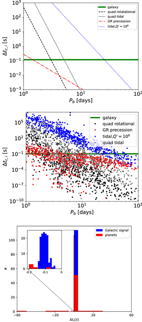
Figure 1. (Top) The shift in the eclipse midpoint time Δtc,i (where i refers to each individual physical acceleration mechanism) over a time baseline of a decade due to individual acceleration mechanisms, assuming low eccentricity (e = 0.01). Here, the shift in the midpoint time due to tidal decay is an upper limit, as we have assumed that the stars are not synchronized. Assuming that the stars are synchronized, this suggests that the effective parameter space for nearly circular EBs corresponds to Pb > 15 days, where other dynamical mechanisms lead to a Δtc,i that is smaller than that produced by the Galactic potential. (Middle) The contributions to Δtc,i for the EBs analyzed by Windemuth et al. (2019). Assuming that the stars are tidally synchronized, there are 230 EBs for which the Galactic signal can be extracted (i.e., for a set, Δtc,quad tidal< 0.1 s; other contaminants to the Galactic signal are subdominant). (Bottom) Histogram showing the contribution to Δtc from a realization of a synthetic population including stars that trace the Galactic signal (blue) and circumbinary planets (red). The level of overlap is minimal, and we can expect that circumbinary planets are not a significant contaminant to the Galactic signal.
Download figure:
Standard image High-resolution imageWe have focused here on eclipse-timing measurements of stellar EBs rather than transiting exoplanets because EBs’ timing precision is generally better due to their deeper eclipses and shorter ingress–egress durations. The timing precision depends linearly on the transit depth, which is proportional to the square of the radius ratio of the two stars. Additionally, the timing precision is proportional to the square root of the ingress–egress durations; these durations are also proportional to the sizes of the stars (Carter et al. 2008; Winn 2010).
2.1. The Accessible Parameter Space for Measuring Galactic Accelerations with Eclipse Timing
Figure 1 (top panel) displays the contributions to the measured shift in EB mideclipse times Δtc,i
due to the various mechanisms discussed above as a function of the binary period for e = 0.01; for simplicity, we consider solar-mass stars with k2,⋆ = 0.016. In calculating the rotationally induced quadrupole moment, we assume Ωi
/n = 1. Here, we have assumed a tidal quality factor  . For small eccentricities, the Galactic signal is measurable for long periods (Pb
> 25 days), even if the stars are not tidally synchronized (N.B. here the contribution shown from tidal decay is an upper limit). Lowering (increasing)
. For small eccentricities, the Galactic signal is measurable for long periods (Pb
> 25 days), even if the stars are not tidally synchronized (N.B. here the contribution shown from tidal decay is an upper limit). Lowering (increasing)  leads to increasing (lowering) the contribution from tidal decay, such that
  gives Δtc,i < 0.1 s for Pb
> 30 days and
gives Δtc,i < 0.1 s for Pb
> 30 days and  gives Δtc,i < 0.1 s for Pb
> 15 days. Also, if the binary has a mildly eccentric orbit, the tidally induced quadrupole moment may lead to a sufficiently large Δtc,i
(see Equation (7)) that we cannot extract the Galactic signal from an analysis of the eclipse midpoint time for shorter periods (Pb
< 20 days). While we may expect statistically that many of the sources at low periods are circularized (Justesen & Albrecht 2021), it is essential to calculate the orbital parameters for individual sources to explicitly check that the Galactic signal can be extracted.
gives Δtc,i < 0.1 s for Pb
> 15 days. Also, if the binary has a mildly eccentric orbit, the tidally induced quadrupole moment may lead to a sufficiently large Δtc,i
(see Equation (7)) that we cannot extract the Galactic signal from an analysis of the eclipse midpoint time for shorter periods (Pb
< 20 days). While we may expect statistically that many of the sources at low periods are circularized (Justesen & Albrecht 2021), it is essential to calculate the orbital parameters for individual sources to explicitly check that the Galactic signal can be extracted.
Windemuth et al. (2019) have recently presented the orbital and stellar parameters for 728 EBs observed by Kepler for which they performed a custom extraction of the light curves. Given their orbital and stellar parameters, we can calculate the contributions to Δtc,i
from the aforementioned effects for these individual systems. We have adopted k2 = 0.016 (Claret 2019) in the calculation of the rotationally and tidally induced quadrupole and have checked that for the set of stars for which these terms are subdominant, the sample is indeed composed of roughly solar-mass stars. The mean and standard deviation of the mass of the primary star for this sample are 1.1 M⊙ and 0.8 M⊙, respectively, and for the secondary star are 0.98 M⊙ and 0.5 M⊙. In Figure 1 (middle) panel, we are showing the maximum possible contribution from  (by assuming synchronization) and
  (by assuming asynchronization). Because we do not have information on the spins of the stars, we cannot say which of these possibilities is realized, but by showing both contributions, we are showing a conservative estimate. Assuming tidal synchronization, we find that there are a large number of EBs (425) that have sufficiently low eccentricities such that the contribution to Δtc,i
from other physical mechanisms is lower than the Galactic acceleration, as shown in Figure 1 (middle panel).
(by assuming asynchronization). Because we do not have information on the spins of the stars, we cannot say which of these possibilities is realized, but by showing both contributions, we are showing a conservative estimate. Assuming tidal synchronization, we find that there are a large number of EBs (425) that have sufficiently low eccentricities such that the contribution to Δtc,i
from other physical mechanisms is lower than the Galactic acceleration, as shown in Figure 1 (middle panel).
Circumbinary planets may also induce a shift in the eclipse midpoint time. Following our earlier work on examining contaminants to the Galactic signal for EPRV surveys (Chakrabarti et al. 2020), we create a synthetic population of stellar binaries and their associated circumbinary planets. We sample from the observed demographics of planets around binary stars, which (in our current understanding) appear to be different from the single-star population in several ways, as found in earlier work (Armstrong et al. 2014; Li et al. 2016; Orosz et al. 2019; Kostov et al. 2021). Circumbinary planets tend to have an average distribution of periods that range from months to years, with essentially no known short-period planets. The upper mass range of circumbinary planets is significantly less than planets orbiting single stars, and they are typically on coplanar orbits relative to the binary.
By sampling from the observed demographics of circumbinary planets, we create a synthetic population of stars and their associated planets and calculate the contribution to Δtc,i from circumbinary planets. Here, we focus on the contribution from planets and the Galactic signal to Δtc,i. By assumption, 50% of the stars in our synthetic population are assigned three planetary companions, leading to a mean number of about two planets per star. We take the Galactic signal to be a Gaussian centered at 0.1 s. The bottom panel of Figure 1 displays a histogram of Δtc,i values induced by circumbinary planets in such a synthetic population. The p-values from the Kolmogorov–Smirnov test for the two distributions corresponding to ±5σ of the mean of the Galactic signal and circumbinary planets that overlap in this range are very small; for a typical realization, the p-value is 10−4 or lower. This indicates that these two populations are distinct and that we can reject the null hypothesis that the signal (the measured Δtc,i) is due to circumbinary planets.
3. Measuring Galactic Accelerations with Kepler EBs
To measure Galactic accelerations over a decade timescale, it is necessary to be able to measure a shift in the eclipse midpoint time to about ∼0.1 s for sources that are at ∼kiloparsec distances from the Sun. We can expect the vertical Galactic acceleration to scale approximately linearly with vertical height; we gave a fitting formula for the vertical dependence in earlier work by analyzing pulsar timing observations (Chakrabarti et al. 2021). This linear dependence is also expected from earlier kinematic analysis (Holmberg & Flynn 2000). We can expect the radial component of the acceleration to scale as  , where Vc
is the circular speed and R is the Galactocentric radius.
, where Vc
is the circular speed and R is the Galactocentric radius.
Using the Kepler EB Catalog (Prša et al. 2011; Kirk et al. 2016), we identified detached EBs with no significant evidence of eccentricity by requiring that the catalog’s morphology parameter morph < 0.5 and primary/secondary eclipse separation parameter 0.49 < sep < 0.51. For each EB, we pulled its long-cadence light curve and observable quantities (e.g., periods and eclipse durations) from the Kepler EB Catalog, and we used the Price & Rogers (2014) relations to estimate the uncertainty on the mideclipse times. These criteria select a sample of 70 detached EBs; for these, we estimate Δtc ≤ 1 s, and we have inspected their light curves by-eye. The Kepler light curves of these sources typically exhibit few-hundred-ppm photometric precision. We used the batman Python package (Kreidberg 2015) to fit transit models to these data; note that we are interested solely in the mideclipse timing for our purposes and not on the accuracy of the recovered physical parameters.
Figure 2 depicts the Galactocentric coordinates for these 70 EBs, which we determine from the Gaia eDR3 data set (Lindegren et al. 2021). We also show here the set of 425 EBs from Windemuth et al. (2019) that have a low enough tidally induced quadrupole moment that the Galactic signal should be measurable. For this set of about 500 sources, about half have timing precision better than 0.5 s. Relative to our pulsar sample (Chakrabarti et al. 2021), there are a significantly larger number of EBs above the Galactic disk and more EBs above the Galactic disk at larger radial distances from the Sun. This suggests that EBs, in addition to pulsars, may allow for a tighter constraint on the Oort limit. In our earlier analysis using pulsar timing, we did not see any clear patterns in the residuals of the measured line-of-sight accelerations at the pulsar locations relative to commonly used static models. The larger number of EBs may manifest clearer residuals (that may arise due to, e.g., out-of-equilibrium effects, dark matter substructure, or a warp or a lopsided mass distribution) in the line-of-sight acceleration.
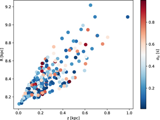
Figure 2. Galactocentric R and z coordinates for the EBs from Windemuth et al. (2019) that have Δtc,quad tidal < 0.1 s and an additional (70) sources from the Kepler Villanova catalog that have low eccentricities (e ∼ 0.01) with timing precision better than 1 s (for reference, the Sun is at R = 8.1 kpc, z = 0.05 pc). The color bar denotes their estimated HST mideclipse timing errors σtc , with bluer colors denoting better precision and redder colors denoting worse precision. We expect HST to measure the mideclipse times to subsecond precision for many of these sources. A precision of ∼0.1 s allows us to measure the Galactic acceleration at ∼kiloparsec distances on a per-star basis, while lower precisions will still allow for statistical measurement.
Download figure:
Standard image High-resolution imageWe note that the uncertainties cited in Windemuth et al. (2019) for the specific set of sources that we consider here (which correspond to sources for which the Galactic potential produces the dominant dynamical effect) typically lead to timing precisions that are about a factor of 2–3 worse than our estimates here. If ∼0.1 s timing precision is not possible on a per-star basis, we should still be able to produce a statistical measurement by increasing our sample size correspondingly (as N2). Follow-up observational work will also require the use of TESS light curves (or other observations after Kepler) to forecast the eclipse times to better than 1 minute eclipse-timing accuracy. Data of eclipsing binaries (Petrosky et al. 2021) from all-sky surveys, such as the time-series component of the Wide-field Infrared Survey Explorer (WISE), may also help to improve the timing precision relative to Kepler observations alone. Indeed, it may be necessary in our follow-up observational work to obtain multiple transits rather than a single transit to obtain the timing precision that we are aiming for.
To demonstrate that 0.1 s eclipse timing is possible in principle with HST, we use PandExo (Batalha et al. 2017) to generate a synthetic HST light curve covering the 25% deep primary eclipse of this bright (K = 11.9; Jmag = 10.93), Pb
= 23 day EB KIC 4144236. With 2 minute exposures, 28 exposures per HST orbit, and 6 orbits, our synthetic light curve has a typical per-point flux precision of 104 ppm; by fitting a batman transit model to it and estimating the timing uncertainty using a Markov Chain Monte Carlo (MCMC) analysis, we are able to determine the mideclipse time to 0.1 s. Figure 3 shows our synthetic light curve, best-fit transit model, and MCMC posterior for  .
.
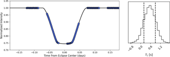
Figure 3. (a) Simulated HST WFC3 primary eclipse light curve of KIC 4144236 (blue points) and the best-fit transit model from batman (Kreidberg 2015; black curve). (b) Posterior distribution for the eclipse midpoint time Tc from the transit modeling, demonstrating that a 0.1 s precision on Tc is achievable with HST.
Download figure:
Standard image High-resolution imageAdditional variability in EB light curves can in principle reduce the accuracy of eclipse-timing measurements. One can account for ellipsoidal variations and rotation signals from the Kepler light curves via, e.g., basis spline fitting (Vanderburg & Johnson 2014). These signals’ timescales are generally long relative to the eclipse durations, so they will manifest as low-order polynomial flux changes in light-curve data. Follow-up spectroscopy and radial velocities can constrain EBs’ eccentricities to <1% and further rule out third bodies that might contribute to eclipse transit viariations (ETVs). Our analysis here, sampling from the observed demographics of circumbinary planets, suggests that dynamic effects from planets would not contaminate the Galactic signal for sufficiently large samples of acceleration measurements. One can estimate (as we have done above for circumbinary planets) the contribution of a third body to ETVs. For the sample of 392 hierarchical triple stellar systems that are resolved by Gaia and have wide separations, the contribution to Δtc,i is much smaller than ∼0.1 s. However, there is also a population of compact triple stellar systems where the magnitude of ETVs is large (Borkovits et al. 2015). Most binaries with P > 10 days do not have tertiary companions (Tokovinin et al. 2006; Tokovinin 2020). To select for sources where other dynamical effects are subdominant, our sources typically have periods larger than 10 days, and we may therefore expect this effect to be small, although any observational follow-up should vet for third light.
These new techniques—pulsar timing, time-domain optical spectroscopy using extreme-precision radial velocity observations or “optical timing,” and eclipse timing—now enable precision measurements for “real-time” Galactic dynamics. Establishing a baseline for distant EBs will prove fruitful for upcoming space-based missions such as Roman, as the signal grows quadratically with time.
4. Conclusion
We summarize our main findings below.
- 1.We show that, in principle, it is now possible to use HST (or other space missions that can achieve comparable photometric precision) of Kepler eclipsing binaries to measure the Galactic acceleration. By measuring an eclipse today, we can detect the ∼0.1 s shift in the midpoint of the eclipse time due to the Galactic gravitational potential. If ∼0.1 s timing precision is not possible on a per-star basis, we should still be able to produce a statistical measurement by increasing our sample size correspondingly (as N2).
- 2.We have analyzed contributions to the period drift rate from sources other than the Galactic potential, including the relativistic precession of an eccentric orbit, tidal decay, and the rotationally and tidally induced quadrupole. Our approach here in modeling these contributions is necessarily approximate due to the uncertainties in modeling tidal decay, and our calculation of the tidal decay contribution is an upper limit assuming the stars are not tidally synchronized. For low periods, there can be significant contributions from the GR precession and the tidally and rotationally induced quadrupole even for low eccentricities.
- 3.We calculate the contributions to the change in the eclipse midpoint time due to these dynamical effects for the sample of EBs analyzed earlier by Windemuth et al. (2019) using their orbital and stellar parameters. For this data set, assuming that the stars are tidally synchronized, there are 425 sources with Δtc,i < the Galactic signal, such that the Galactic acceleration is indeed measurable.
- 4.We create a synthetic population of circumbinary planets by sampling from their observed demographics and calculating their contribution to Δtc,i. We find that there is a sufficiently small overlap with the Galactic signal such that circumbinary planets are not a significant contaminant to the Galactic signal.
- 5.Using analytic relations for the timing precision, we find that there are about 200 EBs in the Kepler field that have timing precision better than 0.5 s and for which all other dynamical effects are subdominant to the Galactic signal. These EBs populate a different region of physical parameter space than the pulsars earlier analyzed by Chakrabarti et al. (2021). We may be able to leverage the size of the larger EB sample (compared to the pulsar sample) to place constraints on nonequilibrium effects and/or dark matter substructure by analyzing residuals in the line-of-sight acceleration relative to static models and to improve the precision of the Oort limit and local dark matter density relative to the earlier pulsar timing analysis.
- 6.We used the EB KIC 4144236 (K = 11.9; Jmag = 10.93) as a worked example, analyzing a simulated HST WFC3 light curve (∼100 ppm flux precision in 2 minutes of exposures) of its 25% deep primary eclipse. The light curve has a photometric precision of 104 ppm, and we are able to constrain the mideclipse time to 0.1 s.
- 7.Unlike kinematic methods, the signal from direct acceleration methods like this one grows with time and, in this case, quadratically with time. Thus, the Galactic signal from EBs for upcoming Roman observations will be substantially larger than what it is today (when the measurement has just become possible), given the baseline established a decade ago by Kepler.
The Center for Exoplanets and Habitable Worlds and the Penn State Extraterrestrial Intelligence Center are supported by the Pennsylvania State University and the Eberly College of Science.
S.C. gratefully acknowledges support from NSF AAG 2009574 and hospitality provided by the CCA at the Flatiron Institute. R.R.R. is supported by STFC grant ST/T00049X/1. We thank N. Sehgal for coining the word “optical timing.” We are grateful to S. Tremaine for helpful comments on the paper and for catching an error on the value of the apsidal motion constant. We thank J. Winn, R. Dawson, G. Ogilvie, A. Prsa, and J. Pepper for helpful discussions and the anonymous referee for helpful comments.
This research has made use of NASA’s Astrophysics Data System Bibliographic Services. This work has made use of data from the European Space Agency (ESA) mission Gaia (https://www.cosmos.esa.int/gaia), processed by the Gaia Data Processing and Analysis Consortium (DPAC, https://www.cosmos.esa.int/web/gaia/dpac/consortium). Funding for the DPAC has been provided by national institutions, in particular the institutions participating in the Gaia Multilateral Agreement.