
Abstract
We present new empirical constraints on the evolution of  , the cosmological mass density of molecular hydrogen, back to z ≈ 2.5. We employ a statistical approach measuring the average observed 850 μm flux density of near-infrared selected galaxies as a function of redshift. The redshift range considered corresponds to a span where the 850 μm band probes the Rayleigh–Jeans tail of thermal dust emission in the rest frame, and can therefore be used as an estimate of the mass of the interstellar medium. Our sample comprises of ≈150,000 galaxies in the UK InfraRed Telescope Infrared Deep Sky Survey Ultra-Deep Survey field with near-infrared magnitudes KAB ≤ 25 mag and photometric redshifts with corresponding probability distribution functions derived from deep 12-band photometry. With a sample approximately 2 orders of magnitude larger than in previous works we significantly reduce statistical uncertainties on
  to z ≈ 2.5. Our measurements are in broad agreement with recent direct estimates from blank field molecular gas surveys, finding that the epoch of molecular gas coincides with the peak epoch of star formation with
  at z ≈ 2. We demonstrate that
  can be broadly modeled by inverting the star formation rate (SFR) density with a fixed or weakly evolving star formation efficiency. This “constant efficiency” model shows a similar evolution to our statistically derived
  , indicating that the dominant factor driving the peak star formation history at z ≈ 2 is a larger supply of molecular gas in galaxies rather than a significant evolution of the SFR efficiency within individual galaxies.
1. Introduction
Three intimately linked observational tracers broadly characterize the cosmic evolution of galaxies: the volume averaged star formation rate (SFR) density  , the stellar mass density
  , and the molecular gas density
  . Our current understanding of galaxy evolution is largely driven by comprehensive measurements of the former two (see Madau & Dickinson 2014 for a review), with a clear empirical picture emerging of an evolution of star formation, which rises rapidly to a peak around z ≈ 2 and then decays to the present day. Completing the triptych is important since the evolution of the molecular gas content of galaxies encodes several important pieces of astrophysics: gas consumption in star formation; gas recycling via feedback; and fresh gas accretion. Ultimately, it is the evolution of molecular gas that drives galaxy evolution as it is the fuel from which stars are assembled. Measurements of molecular gas in galaxies are therefore needed to complete the picture, and to resolve a key outstanding question: Was the peak of star formation history driven by a larger supply of molecular gas or because galaxies formed stars more efficiently (e.g., driven by galaxy mergers/instabilities etc.), or both?
The bulk of the cold gas reservoir in the universe is comprised of hydrogen gas in the form of atomic hydrogen (HI) and molecular hydrogen (H2). In the current model of galaxy formation gas is delivered into galaxies via hot- or cold-mode accretion (e.g., Birnboim & Dekel 2003). The cooling gas must form H2 for star formation to occur. The two main routes to H2 formation in galaxies are via the gas-phase reaction H + e− → H− + γ, H− + H → H2 + e−, and via a dust phase, where H2 forms on the surface of dust grains via efficient three-body reactions (Gould & Salpeter 1963).
H2 radiates poorly in typical interstellar medium (ISM) conditions due to the lack of a permanent dipole moment and a minimum rotational excitation temperature that is significantly higher (≈500 K) than typical temperatures of the cold star-forming ISM (Wakelam et al. 2017). However, H2 can be indirectly traced through its interactions with CO, which traces the same cold, dense ISM and has a low dipole moment enabling its excitation in regions of low density (ncrit ∼ 102 cm−3). Consequently, 12CO, the second most abundant molecule in the ISM, is commonly used as a tracer of the available reservoir of molecular gas in galaxies (e.g., Solomon & Vanden Bout 2005; Carilli & Walter 2013). The ground-state transition CO(J = 1 → 0) is a reliable tracer of total molecular gas, with the conversion factor from CO luminosity to H2 gas mass ( ) calibrated locally (see Bolatto et al. 2013 for a review). Observing the ground-state transition line avoids additional uncertainties inherent in observations of higher-J CO transitions, which require a correction for gas excitation to derive the equivalent CO(J = 1 → 0) luminosity.
Until recently measurements of the cosmological molecular gas mass density were hampered by a paucity of observational data. Over the past few years direct measurements of the cold molecular gas reservoirs of individual galaxies have increased rapidly, with surveys primarily targeting local galaxies (e.g. Keres et al. 2003; Andreani et al. 2020; Fletcher et al. 2020) and star-forming and lensed galaxies (e.g., Frayer et al. 1998, 1999; Coppin et al. 2007; Tacconi et al. 2010; Ivison et al. 2011; Thomson et al. 2012; Bothwell et al. 2013; Riechers et al. 2013; Stach et al. 2017; Oteo et al. 2018; Gómez-Guijarro et al. 2019; Lenkić et al. 2020). However, as these surveys rely on observationally expensive detections of faint spectral lines, measurements of molecular gas mass are still dwarfed in number in comparison to the samples for which SFR and stellar mass estimates are derived. Moreover, to properly assess the cosmological evolution of the cold gas content of galaxies a blank field survey approach is required to measure the gas mass function, rather than targeted (and therefore biased) observations of high-z galaxies as has generally been the case for cold gas observations outside the local volume.
Recently, surveys using a blank field molecular line scan strategy have emerged as an alternative to targeted observations. These surveys evade many of the biases toward massive star-forming galaxies inherent in targeted approaches. The inaugural blank field CO survey employed the Plateau de Bure Interferometer in observations of the Hubble Deep Field North (Decarli et al. 2014; Walter et al. 2014). This was followed more recently by the Atacama Large Millimeter/submillimeter Array (ALMA) Spectroscopic Survey in the Hubble Ultra Deep Field (ASPECS; Aravena et al. 2016a, 2016b; Bouwens et al. 2016; Carilli et al. 2016; Decarli et al. 2016a, 2016b; Walter et al. 2016), the ASPECS Large Program (ASPECS LP; Boogaard et al. 2019; Decarli et al. 2019; González-López et al. 2019; Popping et al. 2019; Decarli et al. 2020), and the CO Luminosity Density at High Redshift survey (COLDZ; Pavesi et al. 2018; Riechers et al. 2019). These surveys have presented results setting out valuable new constraints on the evolution of  over a redshift range 0 ≲ z ≲ 7, obtained through blank field observations of CO line emission. However, due to low number statistics and the small survey areas (which are prone to strong clustering-enhanced sample variance) used to derive the CO luminosity functions, these measurements are hampered by large statistical uncertainties.
To combat the shortfall in direct measurements of molecular gas Scoville (2013), Scoville et al. (2014, 2016, 2017) employed a complementary approach that utilizes submillimeter observations of the long-wavelength dust continuum as a measure of the molecular gas mass in galaxies. The Rayleigh–Jeans (RJ) tail is nearly always optically thin, and consequently measurements of dust emission can be used as a direct probe of molecular gas mass (e.g., Eales et al. 2012; Magdis et al. 2012). While ordinarily a conversion from dust-to-gas mass would require dust emissivity and dust-to-gas abundance to be constrained, Scoville et al. (2014, 2016, 2017) circumvented this by deriving an empirically calibrated RJ luminosity-to-gas mass ratio using CO(J = 1 → 0) and submillimeter continuum observations of a sample of normal star-forming and starburst galaxies at low-z and submillimeter galaxies (SMGs) at high z. This approach requires assumptions about dust temperature and the evolution of the gas-to-dust mass ratio, but provides molecular gas mass (Mmol) estimates within a factor of ≈2 accuracy (e.g., Scoville et al. 2016, hereafter S16; Kaasinen et al. 2019). Since dust continuum measurements can be made in minutes (in contrast to CO line observations which can take multiple hours, e.g., Bothwell et al. 2013; Tacconi et al. 2013) this method can be used to derive molecular gas measurements for much larger samples of galaxies. The S16 RJ luminosity-to-gas mass calibration has been used to estimate the molecular gas mass for ∼700 ALMA-detected galaxies from the Cosmic Evolution Survey (COSMOS) field, with Scoville et al. (2017) deriving molecular gas masses for individual galaxies at redshifts 0.3 < z < 4.5 and Liu et al. (2019) extending this approach to redshifts of z ≈ 6. This method has also been used in combination with stacking methodologies to estimate average molecular gas masses for large samples of galaxies. Millard et al. (2020) used the S16 calibration and applied this to a sample of 63,658 galaxies to derive the gas mass fraction out to z ≈ 5. Magnelli et al. (2020) used a method similar to that of S16 (which was equivalent at solar metallicity) and applied this to a sample of 555 galaxies to derive the molecular gas mass density to z ≈ 3.
In this paper we contribute to the picture of cosmic galaxy evolution by building on the approach of Scoville (2013) and Scoville et al. (2014, 2016, 2017) estimating the evolution of the cosmological mass density of molecular hydrogen to z ≈ 2.5 via the average submillimeter continuum emission of a sample of 150,000 galaxies selected from a deep near-infrared (NIR) survey in the well-studied UKIDSS-UDS field. The Ultra-Deep Survey (UDS) is the deepest component of the UK InfraRed Telescope (UKIRT) Infrared Deep Sky Survey (UKIDSS; Lawrence et al. 2007). We limit our estimate of the molecular gas mass density to z ≈ 2.5 as the S16 calibration has only been shown to be robust out to this redshift. Adopting a statistical approach allows us to take advantage of an NIR selected sample that is an order of magnitude larger than in surveys that measure dust emission (e.g., Scoville et al. 2017; Liu et al. 2019; Magnelli et al. 2020) or CO spectral line emission (e.g., Walter et al. 2016; Decarli et al. 2019; Kaasinen et al. 2019; Riechers et al. 2019) for individual sources. Our method differs from previous stacking approaches (e.g., Magnelli et al. 2020; Millard et al. 2020) as we do not use a combination of spectroscopic and photometric redshifts for our binning. Instead, in the absence of a sample complete with spectroscopic redshifts, we utilize the full photometric redshift probability distribution functions for all our sources. Our method is complementary to previous works in this field (e.g., Liu et al. 2019; Riechers et al. 2019; Decarli et al. 2020; Magnelli et al. 2020) and allows us to reduce the statistical uncertainties on the cosmological molecular gas mass density out to z ≈ 2.5.
This paper is organized as follows: in Section 2, we define the maps and catalogs used; in Section 3, we present a three-dimensional stacking method, which we employ to measure the average (stacked) observed 850 μm flux densities for NIR selected galaxies as a function of redshift; in Section 4, we show that the approach of S16 can be applied to our stacked 850 μm flux densities to derive the cosmological molecular gas density to z ≈ 2.5. We also demonstrate that the cosmic molecular gas density can be broadly modeled by two complementary approaches (i) from the halo mass function assuming a constant halo mass range, and employing stellar-halo mass and ISM-stellar mass ratios, and (ii) inverting the SFR density assuming a constant efficiency model, and in Section 5 we interpret the overall evolution of the cosmic molecular gas mass density in the context of our results and in comparison to previous works. We present our conclusions in Section 6. We assume a Planck 2015 cosmology, where Ωm = 0.31, ΩΛ = 0.69, H0 = 68 km s−1 Mpc−1 (Planck Collaboration et al. 2016), and a Chabrier (2003) initial mass function. The AB magnitude system is used throughout.
2. Data
2.1. Submillimeter Common-User Bolometer Array 2 (SCUBA-2) Cosmology Legacy Survey
The UKIDSS-UDS field was mapped at 850 μm as part of the SCUBA-2 Cosmology Legacy Survey (Geach et al. 2017). The full details of the data collection, reduction, and map properties are given in Geach et al. (2017). Briefly, the beam-convolved map spans approximately 1 deg2 covering the bulk of the multiwavelength coverage of this field, with a uniform (instrumental) noise of σ850 = 0.9 mJy beam−1. Geach et al. (2017) estimated the SCUBA-2 confusion limit to be σconf = 0.8 mJy beam−1. The beam FWHM is approximately 15″, with a full analytic description of the point-spread function (PSF) given by Geach et al. (2017).
2.2. UKIDSS-UDS Ultraviolet–Optical–Mid-IR Imaging and Catalog
The UDS Data Release 11 (DR11) 12-band matched catalog is K band selected with the 95% completeness limit estimated to be KAB = 25 mag. The full details of this catalog will be comprehensively provided in O. Almaini et al. (2021, in preparation) and W. G. Hartley et al. (2021, in preparation), and only a summary is given here. The catalog provides photometry in 12 bands (U, B, V, R,
 ,
,
 , Y, J, H, K, 3.6 and 4.5 μm), where available.
The J, H, and K photometry is taken from the DR11 release of UKIDSS-UDS. The UKIDSS project, described in Lawrence et al. (2007), utilizes the UKIRT Wide Field CAMera (WFCAM; Casali et al. 2007). The photometric system and calibration are outlined in Hewett et al. (2006) and Hodgkin et al. (2009), respectively, and the pipeline processing and science archive are described in M. J. Irwin et al. (2021, in preparation) and Hambly et al. (2008). UKIDSS-UDS covers an area of 0.8 deg2, reaching median depths of J = 25.6, H = 25.1, and K = 25.3 (5σ, AB, estimated from 2″ apertures in source free areas; O. Almaini et al. 2021, in preparation).
The B, V, R,
 , and
, and  optical imaging is from the Subaru/XMM-Newton Deep Survey, which utilizes Suprime-Cam on the Subaru Telescope (Furusawa et al. 2008). U-band data are from the Canada–France–Hawaii Telescope Megacam instrument (O. Almaini et al. 2021, in preparation) and Y-band imaging is obtained from the VISTA Deep Extragalactic Observations survey (VISTA-VIDEO; Jarvis et al. 2013). The InfraRed Array Camera (IRAC) imaging at 3.6 and 4.5 μm is from the Spitzer UKIDSS Ultra Deep Survey (SpUDS; PI Dunlop), combined with deeper data from the Spitzer Extended Deep Survey (SEDS: Ashby et al. 2013). To expand the coverage to outer regions of the field, shallower data are also used from the SIRTF Wide-area InfraRed Extragalactic survey (SWIRE; Lonsdale et al. 2003).
UDS DR11 provides image masks, with masked regions corresponding to image boundaries, artefacts, and bright stars. We employ the UDS binary mask for “good” regions, which has an unmasked area of 0.64 deg2. This binary mask combines the masked regions of the photometry images detailed above (not including the deeper SEDS or SpUDS IRAC images).
We also utilize the subsets feature of the UKIDSS-UDS catalog and for our galaxy sample chose the catalog-defined “good galaxy” subset, which comprises 217,429 sources. These sources have full 12-band photometry and lie within the corresponding “good mask regions, are not cross-talk sources (for which JHK photometry is likely compromised), and are not classified as stars.
UDS DR11 also includes photometric redshifts derived using the code eazy (Easy and Accurate Zphot from Yale; Brammer et al. 2008). To estimate the photometric redshift for each source the 12-band broadband photometry was fit with a spectral energy distribution template producing a redshift probability distribution (W. G. Hartley et al. 2021, in preparation). We utilize both the maximum-likelihood photometric redshifts and redshift probability distributions provided with UDS DR11. eazy performs well compared to other commonly used photometric redshift codes (e.g., zphot, HyperZ, Rainbow; Dahlen et al. 2013), with the resulting normalized mean absolute deviation between eazy derived photometric redshifts and spectroscopic redshifts found to be only σnmad ≈ 0.02 (W. G. Hartley et al. 2021, in preparation).
3. Methods
We employ a three-dimensional stacking approach based on the simultaneous stacking algorithm simstack (presented in detail in Viero et al. 2013). This method allows for the simultaneous fitting of the average observed flux density for multiple populations that contribute to the flux density in the observed map (such as a population of galaxies split into bins of redshift). Importantly, this method takes into account the (usually) large beam in single-dish submillimeter maps with simulations demonstrating that this method returns an unbiased estimate of the average observed flux density for beam sizes ranging from FWHM = 15″–35″ (Viero et al. 2013). This approach also mitigates against boosting of stacking signals from clustered galaxies (e.g., Chary & Pope 2010; Alberts et al. 2014). Our goal is to find the average observed submillimeter flux densities at given redshift intervals for a population of NIR selected galaxies that best fit the observed flux density in the SCUBA-2 map, taking into account the convolution of point sources with the large beam. In this work, rather than binning galaxies by discrete photometric redshift values, we split our sample across redshift intervals according to the redshift probability distribution of each source.
First, we define our sample, performing a selection in observed K band total magnitude, KAB ≤ 25 mag, with the faint end corresponding to the 95% completeness limit of the UKIDSS-UDS catalog, giving us a sample of 153,399 galaxies. At this limiting magnitude, the 95% stellar mass completeness is ≈109.5
M⊙ at z = 2.5 (A. Wilkinson et al. 2021, in preparation). The redshift probability distribution,  , for each source is discretized in bins of Δz (W. G. Hartley et al. 2021, in preparation). We make a completeness correction to the redshift probability distribution of each source, such that
  of a source of magnitude K integrates to C(K)−1, where C(K) is the catalog completeness at K (W. G. Hartley et al. 2021, in preparation). We assume there is no systematic redshift bias in C(K) for this correction.
With the sample defined, we consider a sky model in which each galaxy contributes a flux density that can be described as

where  is the normalized redshift probability distribution function and
  is the flux density “weighting” at redshift z. In practice we have discrete redshift probability distributions defined over R bins such that, for a population of N galaxies, the flux density in the ijth pixel of a map can be written as

Because of the PSF, the flux contribution of each galaxy is distributed over many pixels according to the convolution

In effect, Equation (1) uses  to split each of the N galaxies in our K-selected sample into R redshift bins and assumes that the galaxies in each redshift bin can be represented by an average observed flux density, 〈Sν
(z)〉. This is effectively the “stacked” flux density.
to split each of the N galaxies in our K-selected sample into R redshift bins and assumes that the galaxies in each redshift bin can be represented by an average observed flux density, 〈Sν
(z)〉. This is effectively the “stacked” flux density.
With the model sky defined we consider an optimization problem where the set of average observed flux densities, 〈Sν
(z)〉, per redshift interval in Equation (1) are unknown coefficients. A key decision in defining our sky model is in the binning of  . The UKIDSS-UDS
  are binned in nonlinear steps of 1 + z(n+1) = 1.001(1 + zn
). This would result in hundreds of free parameters across the redshift range of interest, which is computationally impractical as well as unnecessary given the photometric redshift uncertainties. Instead, we bin each
are binned in nonlinear steps of 1 + z(n+1) = 1.001(1 + zn
). This would result in hundreds of free parameters across the redshift range of interest, which is computationally impractical as well as unnecessary given the photometric redshift uncertainties. Instead, we bin each  to Δz = 0.5, giving 20 equally sized bins across the redshift range of 0 < z ≲ 10.
We aim to find the optimal set of average flux densities that minimizes the square of the residual flux between the model in Equation (3) and the observed beam-convolved map, weighted by the noise. We use the Markov Chain Monte Carlo (MCMC) sampler emcee (Foreman-Mackey et al. 2013) to estimate the best-fit flux densities and their uncertainties. We minimize a negative log likelihood  , with

where  is the observed map and σrms is the instrumental noise map. We initialize 1000 “walkers” with an uninformative prior, such that each walker is set with a vector of flux densities (representing Sν
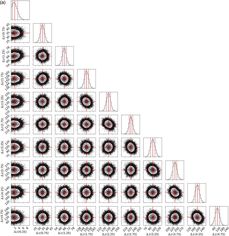
(z)) with each flux density drawn from a Gaussian distribution of mean 0.5 mJy and width 0.05 mJy. The sampler runs for 1000 iterations with the first 500 iterations discarded as burn-in. The best fitting flux densities and the 1σ bounds are estimated from the 16th, 50th and 84th percentiles of accepted samples for 500 iterations. In Figures 1(a)–(c) we show the emcee corner plot of the posterior distributions for all our free parameters.
is the observed map and σrms is the instrumental noise map. We initialize 1000 “walkers” with an uninformative prior, such that each walker is set with a vector of flux densities (representing Sν
(z)) with each flux density drawn from a Gaussian distribution of mean 0.5 mJy and width 0.05 mJy. The sampler runs for 1000 iterations with the first 500 iterations discarded as burn-in. The best fitting flux densities and the 1σ bounds are estimated from the 16th, 50th and 84th percentiles of accepted samples for 500 iterations. In Figures 1(a)–(c) we show the emcee corner plot of the posterior distributions for all our free parameters.
Download figure:
Standard image High-resolution image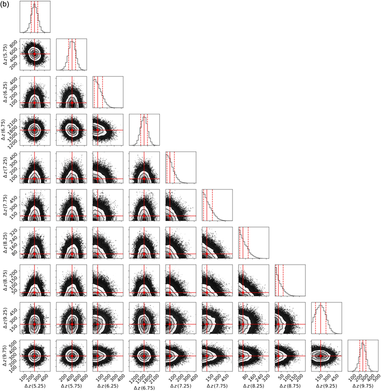
Download figure:
Standard image High-resolution image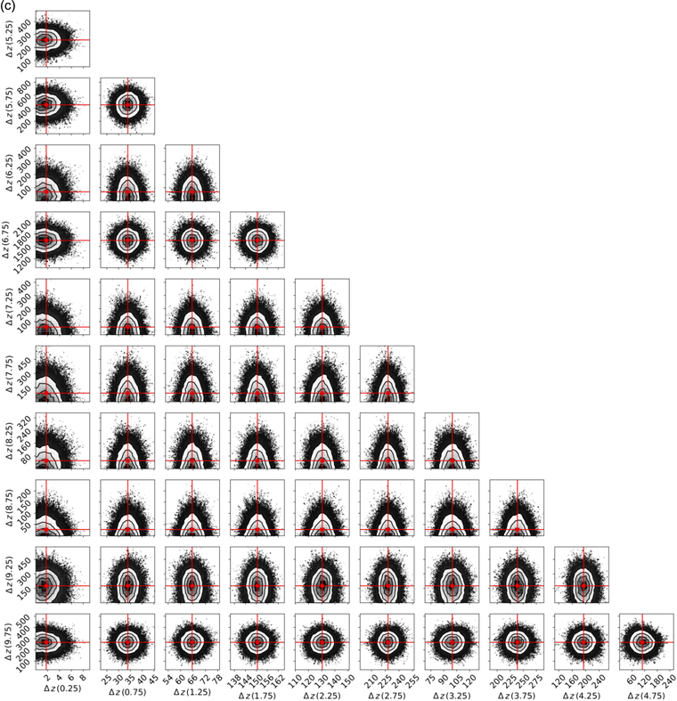
Figure 1. (a) Standard emcee corner plot showing the one- and two-dimensional posterior distributions for our parameters (the average observed flux density in μJy of galaxies in each redshift bin) for the redshift intervals Δz(0.25)–Δz(4.75). The density of the points and the contours correlate with the posterior probability distributions from a 1000-step run (with 500 steps for burn-in discarded) based on our sky model and SCUBA-2 maps, and employing the “delete one” jackknife technique with the map segment area corresponding to A = 1 deleted to take into account sample variance (Tukey 1958). The vertical red lines show the average 850 μm flux density of galaxies for each redshift interval, with the dashed red lines showing the associated 1σ uncertainties (these values are not corrected for the influence of the cosmic microwave background (CMB), see Table 1 for CMB corrected estimates). As evidenced by this plot, there are only very weak correlations between our parameters for the redshifts intervals Δz(0.25)–Δz(4.75). (b) Standard emcee corner plot showing the one- and two-dimensional posterior distributions for our parameters (the average observed flux density in millijanskys of galaxies in each redshift bin) in the redshift intervals Δz(5.25)–Δz(9.75). A detailed description is given in Figure 1(a). As evidenced by this plot there are only very weak correlations between our parameters for the redshifts intervals Δz(5.25)–Δz(9.75). (c) Standard emcee corner plot showing the two-dimensional posterior distributions for our parameters (the average observed flux density in millijanskys of galaxies in each redshift bin) for redshift intervals Δz(0.25)–Δz(4.75) and Δz(5.25)–Δz(9.75). A detailed description is given in Figure 1(a). As evidenced by this plot, there are only very weak correlations between our parameters for the redshifts intervals Δz(0.25)–Δz(4.75) and Δz(5.25)–Δz(9.75).
Download figure:
Standard image High-resolution imageTo estimate the additional uncertainty on the stacked flux densities due to sampling variance we employ the delete one jackknife technique (Tukey 1958), splitting the map into A = 21 approximately equal area sectors and running the MCMC fit for each jackknife. We find that the sampler chains converge quickly (within 200 steps), and the tests indicate that the best-fit parameters are insensitive to the initialization parameters. The covariance matrix is given by

where Sk
i
is the average flux density in the ith redshift bin, eliminating the kth sample and  is the average over all samples. The 1σ uncertainties on the stacked fluxes are estimated by the square root of the diagonal elements of
  .
.
At high z, the increase in the CMB temperature affects the measurement of submillimeter dust continuum in two ways (see da Cunha et al. 2013 for a detailed discussion). First, the CMB provides an additional source of dust heating increasing the intrinsic dust temperature as shown in Equation (6) (da Cunha et al. 2013):

Second, submillimeter observations of dust emission are always measured against the background of the CMB. At low z , Tdust(z) > > Tcmb(z), so essentially all the intrinsic flux is detected against the CMB. However, at high z, as Tcmb(z) approaches Tdust(z), the fraction of submillimeter flux detected against the CMB decreases. Equation (7) (da Cunha et al. 2013) shows the fraction of the intrinsic dust emission from a galaxy measured at a given frequency, vobs = vrest/(1 + z) against the CMB background:

Assuming  K,
K,  (in line with the Tdust adopted in S16) and β = 2, we derive the fraction of submillimeter flux observed against the CMB for the redshift range of 0 < z < 10 at vobs = 353 GHz (λobs = 850 μm), including the extra heating contributed by the CMB. We apply this correction to our average observed 850 μm flux densities in all redshift bins to account for the impact of the CMB on our estimates.
4. Results
4.1. Estimating Molecular Gas Mass: RJ Luminosity-to-gas Mass Relation
In Table 1, we present the average observed 850 μm flux densities for our galaxy sample as a function of redshift. We quote the uncertainties to 1σ and include the additional uncertainty due to sample variance. We note that at z ≳ 6 the UDS redshifts are untested. However, as our sample is binned according to the  for each source, every galaxy effectively contributes to the flux in each redshift interval. Hence, we show the average 850 μm flux density estimates for our galaxy sample to z = 10.
Table 1. Redshift Intervals, Galaxy Weighting in Each Redshift Interval, Average 850 μm Flux Density, and Average 850 μm CMB Corrected Flux Density
| Δz | Galaxy Weighting | 〈S850〉 | CMB Corr. 〈S850〉 |
|---|---|---|---|
| [μJy dz−1] | [μJy dz−1] | ||
| 0.25 | 90003 | 2.1 ± 2.0 | 2.1 ± 2.0 |
| 0.75 | 79917 | 32.9 ± 8.2 | 33.0 ± 8.2 |
| 1.25 | 64475 | 67.5 ± 10.3 | 68.0 ± 10.3 |
| 1.75 | 47922 | 146.9 ± 12.8 | 148.5 ± 12.9 |
| 2.25 | 31448 | 135.0 ± 17.9 | 137.2 ± 18.2 |
| 2.75 | 18368 | 224.9 ± 21.5 | 230.3 ± 22.0 |
| 3.25 | 13071 | 104.6 ± 23.3 | 108.3 ± 24.1 |
| 3.75 | 5271 | 236.5 ± 45.1 | 248.4 ± 47.4 |
| 4.25 | 2413 | 195.0 ± 52.9 | 209.1 ± 56.7 |
| 4.75 | 848 | 130.8 ± 109.6 | 144.3 ± 120.9 |
| 5.25 | 336 | 251.2 ± 109.8 | 288.4 ± 126.1 |
| 5.75 | 79 | 422.9 ± 362.7 | 511.9 ± 439.0 |
| 6.25 | 86 | 74.2 ± 95.7 | 96.2 ± 124.1 |
| 6.75 | 37 | 1606.2 ± 868.8 | 2276.3 ± 1231.3 |
| 7.25 | 49 | 60.2 ± 77.3 | 95.2 ± 122.1 |
| 7.75 | 38 | 106.0 ± 127.0 | 190.8 ± 228.6 |
| 8.25 | 91 | 63.2 ± 73.7 | 132.2 ± 154.1 |
| 8.75 | 121 | 29.0 ± 36.5 | 71.8 ± 90.3 |
| 9.25 | 73 | 155.2 ± 152.5 | 460.6 ± 452.5 |
| 9.75 | 70 | 289.5 ± 161.3 | 1039.0 ± 578.9 |
Note. Column 1: midpoint of each redshift interval (Δz); Column 2: the galaxy weighting, which is the sum of the completeness corrected  in each redshift bin. The summed
  across all redshift intervals integrates to 154,839, which is consistent with the number of galaxies in our sample (153,399) taking into account the completeness corrections; Column 3: average (stacked) 850 μm flux density as a function of redshift with the uncertainty quoted to 1σ; Column 4: average 850 μm flux density corrected for the impact of the CMB as a function of redshift with the uncertainty quoted to 1σ.
Download table as: ASCIITypeset image
We sum  (which is completeness corrected) in each redshift bin, giving us the galaxy weighting for each redshift interval. The integral of the summed
  across all redshift intervals should be approximately equal to the total number of galaxies in our sample. We calculate this to be 154,839, which is consistent with our galaxy sample of 153,399 sources (taking into account the completeness corrections). With the summed
  and taking the area of our sample as the unmasked region of the SCUBA-2 850 μm map (which corresponds to the UDS binary mask for good galaxy regions), we calculate the number density of galaxies as a function of redshift. By combining this with our average flux density (see Table 1, Column 4 for CMB corrected values) we calculate the summed flux density for our galaxy sample in each redshift interval. In Figure 2, we present the number density and summed flux density for galaxies in our sample as a function of redshift. The distribution of the summed flux densities with redshift is broadly comparable to the redshift distribution found for SMGs, which peaks at z ≈ 2 (e.g., Blain et al. 2002; Chapman et al. 2005; Simpson et al. 2014; Miettinen et al. 2017; Zavala et al. 2018), while the number density distribution generally declines with increasing redshift as expected. The difference in the evolution of these distributions demonstrates that our derived flux densities are not biased by the number density of galaxies in each redshift bin.
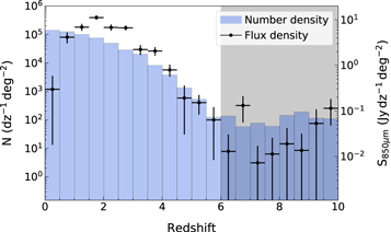
Figure 2. Number density of galaxies in each redshift bin (blue bars) calculated from the galaxy weighting (the sum of the completeness corrected  in each redshift bin) and the area of the unmasked region of the SCUBA-2 image. The black points show the summed flux density of galaxies as a function of redshift derived by combining the number density and the average flux density of galaxies (see Table 1, Column 4 for average flux density values) in each redshift bin. This figure shows the contrasting distributions, with the summed flux density mirroring the redshift distribution found for SMGs with peak at z ≈ 2, whereas the number density generally shows a steady decline. At z ≈ 7, there is an unexpected upturn in the number density and the summed flux density of galaxies, this is likely due to a combination of uncertainties in the photometric redshift fitting at high z (UDS photometric redshifts are untested at z ≳ 6) and the small number statistics in these bins with the galaxy weighting being ≲100 per redshift interval.
Download figure:
Standard image High-resolution imageWe adopt the approach of S16 and utilizing our flux density measurements, estimate the average molecular gas mass for our galaxy sample in each redshift interval. The full details of this approach are given in S16; however, we provide a brief description here.
The long-wavelength RJ tail of dust emission is nearly always optically thin (τ ≪ 1) and consequently this provides a direct probe of the total dust mass and hence the molecular gas mass. S16 utilize this to obtain an empirically calibrated RJ luminosity-to-gas mass ratio

with  . The restriction λrest ≳ 250 μm is required to ensure that at an observed wavelength of 850 μm the rest-frame emission stays on the RJ tail. S16 demonstrated that this luminosity-to-mass ratio is relatively constant for high-stellar mass (Mstellar = (2 − 40) × 1010
M⊙) normal star-forming and star-bursting galaxies, both locally and at high
z.
. The restriction λrest ≳ 250 μm is required to ensure that at an observed wavelength of 850 μm the rest-frame emission stays on the RJ tail. S16 demonstrated that this luminosity-to-mass ratio is relatively constant for high-stellar mass (Mstellar = (2 − 40) × 1010
M⊙) normal star-forming and star-bursting galaxies, both locally and at high
z.
We estimate the average rest-frame 850 μm luminosity density of galaxies as a function of redshift using the average flux densities detailed in Table 1, assuming a mass-weighted dust temperature of 25 K 11 and employing the relation from S16:
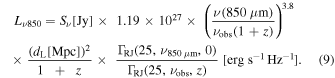
The ΓRJ term in Equation (10) corrects for departures from the RJ ν2 dependence as the observed emission approaches the spectral energy distribution (SED) peak in the rest frame and where Tdust is the mass-weighted temperature characterizing the RJ dust emission

We restrict our estimates of the average rest-frame 850 μm luminosity to z ≲ 2.5 to ensure that rest-frame emission stays on the RJ tail. With the average rest-frame 850 μm luminosity density derived (detailed in Table 2) we use the RJ luminosity-to-gas mass ratio from Equation (8) to estimate the average molecular gas mass as a function of redshift to z ≈ 2.5. This calibration includes a factor of 1.36 to account for the associated mass of heavy elements (mostly helium at 8% by number), so we correct our results by a factor 1/1.36 (Mmol) to obtain  .
.
Table 2. Redshift Intervals, Average Rest-frame 850μ m Luminosity, Average Molecular Gas Mass, Co-moving Molecular Gas Mass Density as a Function of z
| Δz | 〈L850,rest〉 |

|

|

|
|---|---|---|---|---|
| [1027 erg s−1 Hz−1 dz−1] | [107 M⊙ dz−1] | [106 M⊙ Mpc−3] | [10−7] | |
| 0.25 | 1.64 ± 0.02 | 1.80 ± 0.03 | 1.92 ± 1.80 | 115.66 ± 108.42 |
| 0.75 | 81.97 ± 3.89 | 89.95 ± 4.26 | 17.12 ± 4.39 | 569.51 ± 146.13 |
| 1.25 | 217.79 ± 18.32 | 239.01 ± 20.10 | 23.22 ± 4.09 | 430.70 ± 75.93 |
| 1.75 | 514.61 ± 64.72 | 564.77 ± 71.02 | 34.67 ± 5.32 | 380.54 ± 58.41 |
| 2.25 | 492.12 ± 85.19 | 540.08 ± 93.49 | 20.74 ± 4.60 | 143.48 ± 31.84 |
Note. Column 1: midpoint of each redshift interval (Δz); Columns 2 and 3: the average rest-frame 850 μm luminosity and average molecular gas mass for galaxies in each redshift interval; Column 4: molecular gas mass density as a function of redshift and Column 5: molecular gas mass density in terms of the critical mass density. We restrict our results to z ≲ 2.5 to ensure that the observed 850 μm dust emission is tracing the RJ tail.
Download table as: ASCIITypeset image
Since the summed photometric redshift probability distributions inform us about the galaxy weighting in each redshift interval and the UDS binary mask for good regions gives us the unmasked area of the SCUBA-2 850 μm map, we combine this information with the average molecular gas mass and differential co-moving volume element to estimate the co-moving volume density of molecular gas

We present our values for  in Table 2 as a function of redshift, also giving this in terms of the critical mass density
  . We use a Monte Carlo analysis to calculate the uncertainties for our values of L850,rest,
  and
and  , first drawing random values for Sν
from a Gaussian distribution where the mean is the average flux density and width the uncertainty on the average flux density, and then drawing values for a mass-weighted Tdust from a Gaussian distribution with a mean of 25 K (corresponding to the constant Tdust assumed by S16) and width 3 K. Observations (e.g., Planck Collaboration et al. 2011; S16) and simulations (e.g., Liang et al. 2018, 2019) find that a mass-weighted Tdust shows little variation with galaxy L850 or redshift (see Behrens et al. 2018), and by utilizing a temperature distribution with σ = ±3 K, we recognize this minimal variance in our uncertainty calculations. We use these values to estimate L850,rest,
, first drawing random values for Sν
from a Gaussian distribution where the mean is the average flux density and width the uncertainty on the average flux density, and then drawing values for a mass-weighted Tdust from a Gaussian distribution with a mean of 25 K (corresponding to the constant Tdust assumed by S16) and width 3 K. Observations (e.g., Planck Collaboration et al. 2011; S16) and simulations (e.g., Liang et al. 2018, 2019) find that a mass-weighted Tdust shows little variation with galaxy L850 or redshift (see Behrens et al. 2018), and by utilizing a temperature distribution with σ = ±3 K, we recognize this minimal variance in our uncertainty calculations. We use these values to estimate L850,rest,  and
and  from Equations (9), (8), and (11), respectively, for 1000 runs, with the uncertainty being taken as the standard deviation across these trials.
We note that the galaxy sample we use to derive the results in Tables 1 and 2 includes all galaxies in the good galaxy subset of the UDS DR11 catalog, regardless of the reliability of photometric redshifts for individual sources. If we apply a χ2 cut to exclude galaxies with the least reliable redshifts (omitting galaxies with a reduced χ2 value for the photometric redshift of >10) and repeat the process outlined in Sections 3 and 4 above, we find a less than 2% variation in our results with estimates consistent with those in Table 2 within the uncertainties.
We plot  in Figure 3, compared to direct CO line estimates from ASPECS (Decarli et al. 2016b, 2020), COLDZ (Riechers et al. 2019), and VLASPECS (Riechers et al. 2020), as well as values derived using far-IR and UV photometry (Berta et al. 2013). We fit a function of the same form as the SFR density function presented in Madau & Dickinson (2014) to the log of our results, and derive the best-fit parameters for our data using emcee. This yields
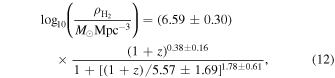
which we plot in Figure 3. Our results show a peak  at z ≈ 2 mirroring existing constraints.
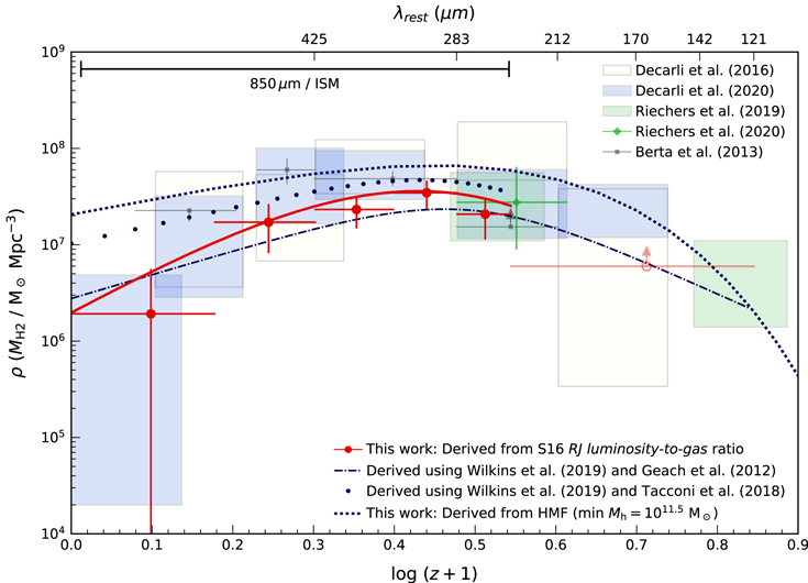
Figure 3. Values for  (CMB corrected) derived using a 3D stacking method and the RJ luminosity-to-gas mass ratio of S16. The upper x-axis shows the rest-frame wavelength of observed 850 μm emission for the redshift range shown, illustrating the range at which rest-frame emission traces the long-wavelength RJ tail (i.e., λrest ≳ 250 μm) and the S16 calibration can be reliably applied. Our estimates are represented by the red points (uncertainties shown to 2σ) with the solid red line showing the best-fit function derived using emcee and a function of the same form as the SFR density function from Madau & Dickinson (2014). We note that at z ≳ 2.5 our results should be considered speculative as the observed 850 μm emission no longer traces the rest-frame RJ tail. Hence, we only show an average of our estimates after this point. We do not include any estimates for z ≳ 6 as the UDS photometric redshifts beyond this are untested and as such highly uncertain. Alongside our values we show results from ASPECS (off-white rectangles; Decarli et al. 2016b), ASPECS LP (blue rectangles; Decarli et al. 2020), COLDz (green rectangles; Riechers et al. 2019), and VLASPECS (green diamond; Riechers et al. 2020), which are derived from direct measurements of CO line emission. The gray points show values from Berta et al. (2013), estimated using deep far-IR and UV data, and assuming either typical gas depletion times (Tacconi et al. 2013) or from IR luminosity and obscuration properties (Nordon et al. 2013). We plot our constant efficiency models derived using the recalibrated star formation history from Wilkins et al. (2019) and assuming either a corresponding constant (e.g., Geach & Papadopoulos 2012) or weakly evolving (e.g., Tacconi et al. 2018) volume averaged star formation “efficiency” to infer
  . The former is shown as the dark blue dotted–dashed line and the latter illustrated by the dark blue circles. We also plot
  to z ≈ 7 derived from the halo mass function (Murray et al. 2013), assuming the stellar-halo mass ratio from Moster et al. (2013) and ISM-stellar-mass relation from Scoville et al. (2017). The dark blue dotted line corresponds to a halo mass range of 1011.5–1015
M⊙, with the minimum stellar masses derived for this range (≈109.5
M⊙) being consistent with the lowest stellar masses probed in ASPECS LP (Boogaard et al. 2019).
to z ≈ 7 derived from the halo mass function (Murray et al. 2013), assuming the stellar-halo mass ratio from Moster et al. (2013) and ISM-stellar-mass relation from Scoville et al. (2017). The dark blue dotted line corresponds to a halo mass range of 1011.5–1015
M⊙, with the minimum stellar masses derived for this range (≈109.5
M⊙) being consistent with the lowest stellar masses probed in ASPECS LP (Boogaard et al. 2019).
Download figure:
Standard image High-resolution image4.2. Deriving Molecular Gas Mass Density from the Halo Mass Function
Using an alternative approach we derive  from first principles using the halo mass function from Murray et al. (2013) and assuming a constant halo mass range of 1011.5–1015
M⊙. We estimate the molecular gas mass density as a function of halo mass (for redshifts 0 ≤ z ≤ 7) using the stellar-halo mass ratio from Moster et al. (2013) and the ISM-stellar mass relation from Scoville et al. (2017). The ISM-stellar mass relation is calibrated using a sample of high mass galaxies (Mstellar ≳ 1010
M⊙), therefore, we adopt a halo mass range for which the corresponding stellar masses are comparable with the Scoville et al. (2017) calibration sample. Integrating these estimates with respect to halo mass gives the total molecular gas density as a function of redshift, which we present in Figure 3.
from first principles using the halo mass function from Murray et al. (2013) and assuming a constant halo mass range of 1011.5–1015
M⊙. We estimate the molecular gas mass density as a function of halo mass (for redshifts 0 ≤ z ≤ 7) using the stellar-halo mass ratio from Moster et al. (2013) and the ISM-stellar mass relation from Scoville et al. (2017). The ISM-stellar mass relation is calibrated using a sample of high mass galaxies (Mstellar ≳ 1010
M⊙), therefore, we adopt a halo mass range for which the corresponding stellar masses are comparable with the Scoville et al. (2017) calibration sample. Integrating these estimates with respect to halo mass gives the total molecular gas density as a function of redshift, which we present in Figure 3.
4.3. Estimating Molecular Gas Mass Density Using a Constant Efficiency Model
We also estimate  from the SFR density,
  , assuming a corresponding volume averaged star formation efficiency,
  . We use the functional fit of Wilkins et al. (2019), a recalibration of the well-known Madau & Dickinson (2014) cosmic star formation history. We make the assumption that η(z) is constant and that the total molecular gas mass per galaxy can be related to ongoing star formation as
  (Geach & Papadopoulos 2012). Here, ξ is the ratio of dense, actively star-forming molecular gas to the total molecular reservoir with ξ ≈ 0.04 for quiescent disks and ξ > 0.5 for starbursts (e.g., Papadopoulos & Geach 2012), while the factor
 describes the rate at which the dense molecular gas forms stars. Figure 3 shows the predicted
 inferred from the Wilkins et al. (2019) fit, assuming a constant “average” η(z) = 0.3 Gyr corresponding to ξ = 0.1 and
 = 37 Gyr−1 (e.g., Geach & Papadopoulos 2012).
This value for η(z) is similar to the typical values of tdep ( ) ≈1 Gyr (e.g., Tacconi et al. 2018) for main-sequence galaxies. Tacconi et al. (2018) found a relatively weak dependence of tdep with redshift, tdep ∝ (1 + z)−0.57 to z < 2.5, consistent with our picture of a common mode of star formation in normal galaxies, at least out to the peak epoch. We use this relation from Tacconi et al. (2018) and the Wilkins et al. (2019) fit to derive an estimate of
  , which incorporates a weakly evolving star formation efficiency. We present our predicted
  in Figure 3.
5. Discussion
Our results appear to be in reasonable agreement with existing empirical constraints, indicating that the epoch of molecular gas coincided with the peak epoch of star formation at z ≈ 2 . So what does this mean in terms of the evolving molecular gas budget? We might ask what is the complete picture of  , or rather, what galaxies host the majority of the cosmic molecular gas budget across cosmic time? In the following discussion, we interpret the overall evolution of the cosmic molecular gas density, in the context of our results, within the established framework of star formation in galaxies from the cosmic dawn to the present day.
5.1. Evolution of Cosmic Molecular Gas Mass Density at 0 ≤ z ≤ 2.5
The S16 RJ luminosity-to-gas mass ratio has been shown to provide molecular gas mass estimates accurate to within a factor of around 2 when compared with measurements made via direct CO ( J = 1 → 0) line observations (e.g., Scoville et al. 2017; Kaasinen et al. 2019), with variations in the dust emissivity index, temperature, and gas-to-dust ratios being accountable for the deviations. This factor of 2 accuracy is based on samples of galaxies with high-stellar masses Mstellar = (2–40) × 1010 M⊙ as these galaxies are likely to have near-solar metallicity (Tremonti et al. 2004). This avoids probing low metallicity sources for which the dust-to-gas abundance ratio is likely to drop or the CO gas fraction is low (Bolatto et al. 2013). In Figure 4, we show the marginalized stellar mass estimates for UDS galaxies (O. Almaini et al. 2021, in preparation) and the corresponding 95% stellar mass completeness (derived using the method of Pozzetti et al. 2010, A. Wilkinson et al. 2021, in preparation) for the UDS catalog. As can be seen in Figure 4, our galaxy sample includes a proportion of galaxies with stellar masses lower than those used to derive the S16 RJ luminosity-to-gas mass ratio, with these sources being more abundant in lower redshift bins.
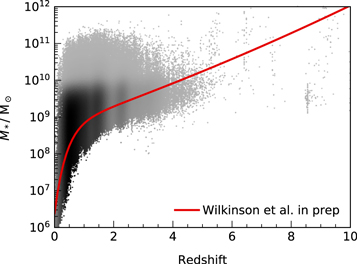
Figure 4. Marginalized stellar mass estimates (O. Almaini et al. 2021, in preparation) for UDS galaxies in our sample as a density plot, with darker colors corresponding to higher number densities of galaxies. The red line corresponds to the UDS catalog 95% stellar mass completeness (derived using the method of Pozzetti et al. 2010, see A. Wilkinson et al. 2021, in preparation). This figure demonstrates that at high redshifts we are only sensitive to the most massive galaxies.
Download figure:
Standard image High-resolution imageThe dust-to-gas relation has been found to be relatively consistent for nearby galaxies with Mstellar > 109 M⊙ (e.g., Groves et al. 2015), but drops for galaxies with lower stellar masses (hence lower metallicities). Cosmological galaxy formation simulations have shown that deviations from this relation become significant (≳0.5 dex) at L850 ≲ 1028 erg s−1 Hz−1 in the redshift range of 0 < z < 9.5 (e.g., Privon et al. 2018). As shown in Figure 4, at z ≳ 1 the majority of our sample are likely to have Mstellar > 109 M⊙ and Table 2 shows that the mean rest-frame 850 μm luminosity for our sample in all but the lowest redshift interval (Δz = 0.25) is L850 μm ≳ 1028 erg s−1 Hz−1. Therefore, while the RJ luminosity-to-gas mass ratio has been calibrated on high-stellar mass galaxies (Mstellar = (2 − 40) × 1010 M⊙), we make the assumption that applying this calibration to our sample at redshifts z ≳ 0.5 is likely to result in comparable uncertainties (i.e., a factor of 2). However, in the redshift bin Δz = 0.25 the mean rest-frame luminosity is 〈L850 μm〉 = 1.6 × 1027 erg s−1 Hz−1, and as such, our results are likely to be underpredicted by ≳0.5 dex (e.g., Privon et al. 2018) due to the abundance of lower mass (low metallicity) galaxies in this redshift interval.
5.2. Comparison of the Evolution of Molecular Gas Mass Density to Other Studies in the Literature
In Figure 3, we compare our results, which are revised to account for the influence of the CMB, to those from direct CO line surveys (e.g., Decarli et al. 2016b, 2020; Riechers et al. 2019, 2020). We limit our discussion to the results from these surveys at z ≲ 2.5 as we are restricted to this redshift range due to the wavelength of our observations (λobs = 850 μm). While the results from ASPECS/ASPECS LP (Decarli et al. 2016b, 2020) and COLDz (Riechers et al. 2019, 2020) were not corrected for the influence of the CMB, we note that this is not necessary at z ≲ 4.5 as the effect of the CMB on measurements of molecular gas mass density from direct CO line observations is minimal (≲15%, e.g., Decarli et al. 2019) and as such this does not impact on our analysis here.
We find that our results are broadly consistent with the estimates from direct CO line surveys within uncertainties and show notably good agreement with results obtained through observations of the ground-state CO line (ASPECS LP at Δz ≃ 0.25 and COLDZ at Δz ≃ 2.25). Albeit, we caution that our results at Δz ≃ 0.25 are likely underestimated due to the abundance of low stellar mass galaxies in this redshift bin.
When compared with the ASPECS LP survey (Decarli et al. 2020) our results generally trace the lower boundaries of their estimates between 0.75 ≲ z ≲ 1.75. The S16 RJ luminosity-to-gas mass ratio is calibrated using the ground-state CO( J = 1 → 0) line, whereas at z > 0.75 the ASPECS LP results are derived from observations of higher state excitation CO lines. Therefore, this offset could be explained by the uncertainties associated with translating higher excitation CO lines observations to ground-state CO( J = 1 → 0) luminosities. However, in the redshift interval Δz = 1.25, even if the extreme case of thermalized gas is assumed, our upper estimate (taking into account 1σ uncertainties) falls a factor of 1.42 below the lower boundary of the ASPECS LP survey (e.g., 38.90 × 10⁶ M⊙ Mpc−3, Table A3, Decarli et al. 2019). As such the uncertainties in CO line ratios do not fully account for the offset we see.
Building on previous studies, Liu et al. (2019) derived the molecular gas mass density using a data set comprised of ≈700 ALMA continuum detected galaxies and ≈1000 galaxies with CO observations (taken from the literature). To derive molecular gas masses for the continuum detected galaxies Liu et al. (2019) employed the Hughes et al. (2017) luminosity-to-gas mass calibration. Liu et al. (2019) estimated an SMF (stellar mass function) integrated molecular gas mass density based on the SMF integrated to Mstellar = 109 M⊙ and using a gas fraction function derived from their composite sample of ≈1700 galaxies. Their results trace the upper boundaries of the molecular gas mass density derived from the most recent blank field CO line surveys (e.g., Decarli et al. 2019; Riechers et al. 2019) and are ≈1 dex higher than our estimates. This offset with our estimates of molecular gas mass density could be in part due to assumptions made in Liu et al. (2019) to derive an SMF integrated molecular gas mass density (i.e., that all star-forming galaxies are on the main sequence) or potentially differences in sample selection. The majority (≈800) of the CO detected sources in the Liu et al. (2019) composite sample are in the local universe (i.e z < 0.3), so at z > 0.3 their data set is dominated by ALMA continuum detected galaxies, which are preferentially massive and dust rich (and hence, using a dust-to-gas mass conversion, gas rich). In contrast our galaxy sample is NIR selected and as such our selection is less likely to sample these luminous dust-rich SMGs, with previous studies finding that ≈20% of SMGs are missed in optical/new-IR surveys (e.g., Dudzevičiūtė et al. 2020). Magnelli et al. (2020) use a stacking approach to measure the co-moving gas mass density of a sample of 555 NIR selected galaxies, with galaxies split into bins of z and Mstellar. Their stacking method accounts for the metallicity of galaxies in these bins (inferred using the stellar mass–metallicity from Tacconi et al. 2018) and is equivalent to the S16 calibration at solar metallicity. Our results trace the lower boundaries of their estimates, but are inconsistent (within 1σ uncertainties) at z > 1. This discrepancy may be in part due to our method not accounting for the metallicity of low mass galaxies, resulting in an underestimation of the molecular gas mass for galaxies with Mstellar < 109 M⊙. However, if this was the sole reason for the difference in our results, we would expect this to have more of an impact at z < 1 where this effect will be more prominent. We caution that our results also rely solely on photometric redshifts, which despite the high-quality 12-band photometry of the UDS catalog, cannot compete with the accuracy of redshifts derived via spectroscopic surveys. By utilizing the redshift probability distributions in our 3D stacking approach, we aim to provide mitigation against these uncertainties. However, while our estimates rely exclusively on the use of photometric redshifts, the results obtained in both ASPECS LP (Decarli et al. 2020; Magnelli et al. 2020) and Liu et al. (2019) benefit from the inclusion of sources with more reliable spectroscopic redshifts. This may also play a part in deviations seen when we compare our estimates with these previous surveys.
5.3. Contribution of the Brightest Submillimeter Sources to the Cosmic Evolution of the Molecular Gas Mass Density
In order to present the most complete view of the evolution of the molecular gas mass density, we stack all sources in our NIR selected sample, including counterparts, to the bright submillimeter sources in the SCUBA-2 UDS map. To test the contribution of these galaxies to our results, we repeat our stacking analysis with the SCUBA-2 UDS source subtracted map. As expected excluding the ∼1000 UDS submillimeter sources reduces the average observed 850 μm flux in our redshift intervals, which propagates to our estimate of the co-moving molecular gas mass density. At z < 1.5 the exclusion of the UDS submillimeter sources has a minimal impact on our estimates of  and these remain consistent within the 1σ uncertainties. However, at z > 1.5 our estimates of
  drop by a factor of 2.05 and 2.33 in the redshift intervals Δz = 1.75 and Δz = 2.25, respectively. This coincides with the peak number density of SMGs at z ≈ 2. This indicates that approximately 50% of the molecular gas mass density at the peak of the SFR density is locked in dust-rich SMGs. We note that our inferred contribution of SMGs is also likely underestimated as we expect that approximately 20% of SMGs are undetected in our NIR selected sample (e.g., Dudzevičiūtė et al. 2020). Our finding is in keeping with that of Zavala et al. (2021) who found that bright SMGS (LIR > 1012
L⊙) dominate the obscured SFR density at z ≈ 2 and also Magnelli et al. (2020) who found that the bulk of dust and gas in galaxies is locked in massive star-forming galaxies.
drop by a factor of 2.05 and 2.33 in the redshift intervals Δz = 1.75 and Δz = 2.25, respectively. This coincides with the peak number density of SMGs at z ≈ 2. This indicates that approximately 50% of the molecular gas mass density at the peak of the SFR density is locked in dust-rich SMGs. We note that our inferred contribution of SMGs is also likely underestimated as we expect that approximately 20% of SMGs are undetected in our NIR selected sample (e.g., Dudzevičiūtė et al. 2020). Our finding is in keeping with that of Zavala et al. (2021) who found that bright SMGS (LIR > 1012
L⊙) dominate the obscured SFR density at z ≈ 2 and also Magnelli et al. (2020) who found that the bulk of dust and gas in galaxies is locked in massive star-forming galaxies.
5.4. Additional Constraints on the Evolution of Molecular Gas Mass Density
We have added further valuable constraints to this picture of cosmic molecular gas evolution using two alternative approaches.
We estimate  from the halo mass function (Murray et al. 2013) assuming a constant halo mass range of 1011.5–1015
M⊙, and using the stellar–halo mass ratio from Moster et al. (2013) and the ISM–stellar mass relation from Scoville et al. (2017). For the latter relation we make the assumption that all galaxies are on the star-forming main sequence (e.g., sSFR/sSFRMS = 1). The evolution of our halo mass derived
from the halo mass function (Murray et al. 2013) assuming a constant halo mass range of 1011.5–1015
M⊙, and using the stellar–halo mass ratio from Moster et al. (2013) and the ISM–stellar mass relation from Scoville et al. (2017). For the latter relation we make the assumption that all galaxies are on the star-forming main sequence (e.g., sSFR/sSFRMS = 1). The evolution of our halo mass derived  (shown in Figure 3) follows a similar shape to the SFR density, rising to a peak at 1 ≲ z ≲ 3 and decreasing to the present day. The minimum halo mass we assume corresponds to stellar masses of ≈109.5
M⊙ (e.g., Moster et al. 2013), equivalent to the lowest stellar masses probed in the ASPECS LP survey (Decarli et al. 2020). Our
(shown in Figure 3) follows a similar shape to the SFR density, rising to a peak at 1 ≲ z ≲ 3 and decreasing to the present day. The minimum halo mass we assume corresponds to stellar masses of ≈109.5
M⊙ (e.g., Moster et al. 2013), equivalent to the lowest stellar masses probed in the ASPECS LP survey (Decarli et al. 2020). Our  estimates show good agreement with the ASPECs/ASPECS LP surveys (Decarli et al. 2016a, 2020) at z ≳ 0.6. However, as shown in Figure 3 at z ≲ 0.6 our estimate of
  lies above the lowest redshift bins from the ASPECS LP survey (Decarli et al. 2020) and is ≈1 dex higher than our estimate of
  derived from measurements of observed 850 μm flux. To obtain an estimate of
  from the halo mass function we make the assumption that all galaxies are star-forming. As such our estimate of
  derived from the halo mass function can be seen as an upper limit
  for the stellar mass range sampled. It follows that we see a more significant deviation between our estimate and observationally derived results at lower redshifts as the fraction of passive galaxies is higher at later epochs.
We also estimate  from the SFR density (Wilkins et al. 2019), assuming a constant (Geach & Papadopoulos 2012) and weakly evolving (Tacconi et al. 2018) star formation efficiency. These constant efficiency models predict a co-moving molecular gas mass density in good agreement with both measurements of molecular gas mass via observations of direct CO line emission (Decarli et al. 2016b, 2020; Riechers et al. 2019, 2020) and our results derived from measurements of the long-wavelength dust emission, out to a peak at z ≈ 2. A simple conclusion is that the peak epoch of star formation at z ≈ 2 is not driven by significantly more efficient (or starburst-like) star formation in galaxies, but by a higher abundance of molecular fuel in galaxies. We note that the estimate derived from weakly evolving star formation is ≈1 dex higher than our results at Δz ≃ 0.25. This is likely a consequence of the latter being underestimated due to the abundance of low stellar mass galaxies in this redshift bin.
We recognize that our assumption of a constant efficiency model is at odds with Scoville et al. (2017), who argued that while cold molecular gas reservoirs increase with z (as (1 + z)1.84), the SFR increases more rapidly (as (1 + z)2.9), indicating that the peak of star formation is a consequence of both increased molecular gas content in galaxies and higher star formation efficiency. We also note that at z ≳ 1 early-type galaxies have been shown to be more compact for a given stellar mass than their local counterparts (e.g., Daddi et al. 2005; Cappellari et al. 2009), which taken in combination with the “Kennicutt–Schmidt” relation (a power-law relation between SFR and gas surface densities, Schmidt 1959; Kennicutt 1998) implies that star formation may be more efficient at z ≳ 1.
The 3D stacking approach we use derives the average properties for galaxies in our sample as a function of redshift, and thus we do not measure the molecular gas mass and SFRs for individual sources. While the UDS DR11 catalog does include Mstellar estimates (which are evaluated at the peak maximum-likelihood redshift) for individual galaxies, our 3D stacking method bins galaxies according to the discretized redshift probability distribution ( ), and as such each galaxy in our sample effectively contributes to the flux in all redshift intervals. Hence, using this 3D stacking method precludes a Mstellar selection relative to our redshift bins. Therefore, we are not able to repeat the analysis from Scoville et al. (2017) to test their assertion of an evolving star formation efficiency.
5.5. The Epoch of Molecular Gas
Although we cannot quantify the contribution of higher star formation efficiencies to the peak of SFR density at z ≈ 2, the symmetry between our constant efficiency models with our statistically derived  indicates a star formation history that is predominantly driven by an increased supply of molecular gas in galaxies, rather than a significant evolution in star formation efficiency (consistent with the findings of Decarli et al. 2020; Magnelli et al. 2020). With this in mind we now turn to the formation of H2 itself. Cazaux & Spaans (2004) combined a microscopic model for the relative rates of gas-phase and dust H2 production with a cosmological model to show the more efficient dust-phase production becomes the dominant route to H2 formation at z ≈ 3–6 for reasonable assumptions about the conditions of the ISM of early galaxies. Therefore, there is a perfect storm for massive galaxy growth at z ≈ 2: not only is the cosmic accretion rate at its peak, massive halos have had time to grow, galaxies have increased gas densities, and previous generations of stars in the progenitors of these systems have provided the metal enrichment that accelerates the formation of H2, which as the fuel for star formation, drives galaxy growth; this could be described as the epoch of molecular gas.
5.6. Estimating the Evolution of Cosmic Molecular Gas Mass Density at z ≳ 2.5
S16 intentionally restricted their calibration sample to galaxies at z ≤ 3 to ensure observed 850 μm emission was from the rest-frame long-wavelength RJ tail, where dust is optically thin and emission is dominated by the contribution of cold dust (which is well represented by a mass-weighted Tdust = 25 K). In Figure 3 we have shown an average of our  estimates at 2.5 ≲ z ≲ 6 (the UDS redshifts are untested at earlier epochs as there are no UDS galaxies with spectroscopic redshifts at z ≳ 6.5), but note that at these redshifts estimates are less reliable due to large uncertainties in the RJ correction (see Equation (10)) as rest-frame emission approaches the peak of the SED.
In the optically thick regime (as rest-frame dust emission moves off the long-wavelength RJ tail) the rest-frame emission no longer correlates with the total dust mass of a galaxy and probes only the surface dust, which using the approach of S16 would result in an underestimation of L850 and hence the molecular gas mass. However, as the rest-frame emission approaches the peak of the SED we are increasingly sensitive to the dense, warm dust component, which significantly boosts the luminosity (with only a small mass fraction) and dominates the emission close to the SED peak. Consequently, rest-frame dust emission at high z is not well represented by a mass-weighted Tdust = 25 K, which would result in an overestimate of the dust and gas mass.
In addition to these competing effects, we are also likely to be missing a significant population of lower mass galaxies at z > 2.5. As shown in Figure 4, the 95% stellar mass completeness at z ≈ 2.5 is predicted to be ≃109.5 M⊙, so we are are simply not sensitive to the majority of low mass galaxies at the highest redshifts. In addition, although relatively rare (with number counts N( > 3.5 mJy) ≃ 3000 deg−2; Geach et al. 2017) SMGs are dust rich (Mdust ∼ 109 M⊙; e.g., da Cunha et al. 2015; Magnelli et al. 2019) and about 20% are undetected in optical/NIR surveys (e.g., Dudzevičiūtė et al. 2020). This non-detection of SMGs is unlikely to have a significant impact on our estimates at low z. However, at z ≳ 2.5 since we are significantly under-sampling the galaxy population and as the number of galaxies in our redshift bins fall the non-detection of dust-rich SMGs becomes more statistically significant, further contributing to an underestimation of the molecular gas mass density at z ≳ 2.5.
The overall impact of the above is difficult to quantify. However, as shown by Figure 3 our results at z ≳ 2.5 are systematically lower than the estimates obtained via direct CO line emission, which suggests that the use of this method past z ≈ 2.5 (when λobs = 850 μm no longer probes the rest-frame RJ tail) results in an underestimation of the molecular gas mass density. In consequence, while our results are highly uncertain at z > 2.5, we suggest that to z ≲ 6 these can be seen as providing a lower limit to the molecular gas mass density.
6. Conclusions
We employ a three-dimensional stacking method (Viero et al. 2013) and an empirically calibrated RJ luminosity-to-gas mass ratio S16 to derive the average molecular gas mass as a function of redshift utilizing a sample of ≈150,000 galaxies in the UKIDSS-UDS field. By combining these techniques we are able to reduce the statistical uncertainties on the evolution of the molecular gas mass density,  , within the redshift range 0.5 ≲ z ≲ 2.5. We find that:
- 1.
 shows a clear evolution over cosmic time which traces that of the SFR density with a peak ≈2 × 10⁷
M⊙ Mpc−3 at z ≈ 2.
shows a clear evolution over cosmic time which traces that of the SFR density with a peak ≈2 × 10⁷
M⊙ Mpc−3 at z ≈ 2. - 2.Our results are consistent with those of blank field CO line surveys, albeit our estimates are systematically lower than those derived using observations of higher excitation CO lines. This may in part be a consequence of the line ratios used to translate higher excitation CO line luminosity to ground-state CO line luminosity.
- 3.Our results are an order of magnitude lower than those derived by Liu et al. (2019), who used the Hughes et al. (2017) luminosity-to-gas mass calibration to estimate molecular gas masses for the ALMA continuum detected galaxies in their sample. This difference in results may be in part due to selection effects, as their ALMA-selected sample preferentially selects dust-rich (and consequently gas-rich) sources, whereas by using an NIR selection we are likely to miss ≈20% of these dust-rich SMGs.
- 4.
- 5. can be derived from first principles from the halo mass function (Murray et al. 2013) in conjunction with stellar-halo mass (Moster et al. 2013) and ISM-stellar mass ratios (Scoville et al. 2017). To obtain this estimate we make the assumption that all galaxies are star forming and hence this can be seen as an upper limit for with respect to the stellar mass range sampled.


We have demonstrated that by applying a statistical method and the approach of S16 we can provide robust, statistically significant constraints to the cosmological gas mass density to z ≲ 2.5. Our results show an evolution that mirrors that of the SFR density, indicating that the peak of the star formation history is primarily driven by an increased supply of molecular gas rather than a significantly increased star formation efficiency. We have shown that at z ≳ 2.5, we detect dust emission from high mass galaxies, even with our NIR selected sample. Hence, in the future there is potential for this approach to be extended to provide improved constraints at higher z through 1 mm/3 mm wide-field surveys with facilities such as the Large Millimeter Telescope.
T.K.G. acknowledges support from a UK Science and Technology Facilities Council studentship. T.K.G also acknowledges support from the Bell Burnell Graduate Scholarship Fund (BB001). K.E.K.C. is supported by a Royal Society Leverhulme Senior Research Fellowship (SRF/R1/191013). K.E.K.C. and M.F. acknowledge the support from STFC (grant No. ST/R000905/1). J.E.G. is supported by a Royal Society University Research Fellowship. C.C.L. acknowledges support from the Royal Society under grant RGF/EA/181016. M.P.K. acknowledges support from the First TEAM grant of the Foundation for Polish Science No. POIR.04.04.00-00-5D21/18-00. M.P.K. also acknowledges support from the Polish National Agency for Academic Exchange under grant No. PPI/APM/2018/1/00036/U/001. The James Clerk Maxwell Telescope has historically been operated by the Joint Astronomy Centre on behalf of the Science and Technology Facilities Council of the United Kingdom, the National Research Council of Canada, and the Netherlands Organisation for Scientific Research. The S2CLS map data were taken as part of Program ID MJLSC02. Additional funds for the construction of SCUBA-2 were provided by the Canada Foundation for Innovation. The UKIDSS project is defined in Lawrence et al. (2007). Further details on the UDS can be found in O. Almaini et al. (2021, in preparation). UKIDSS uses the UKIRT WFCAM (Casali et al. 2007). The photometric system is described in Hewett et al. (2006), and the calibration is described in Hodgkin et al. (2009). The pipeline processing and science archive are described in M. J. Irwin et al. (2021, in preparation) and Hambly et al. (2008).
Footnotes
- 11