INITIAL PLANETESIMAL SIZES AND THE SIZE DISTRIBUTION OF SMALL KUIPER BELT OBJECTS

Hilke E. Schlichting; Cesar I. Fuentes; David E. Trilling

doi:10.1088/0004-6256/146/2/36

1. INTRODUCTION

The Kuiper Belt consists of a disk of icy objects located just beyond the orbit of Neptune. In the Kuiper Belt, planet formation never proceeded all the way to completion, which makes it an ideal laboratory for testing planet formation theories.

The Kuiper Belt size distribution contains many important clues concerning the formation of Kuiper Belt Objects (KBOs), their effective strength, and their collisional evolution (Dohnanyi 1969; Davis & Farinella 1997; Kenyon & Luu 1999; Pan & Sari 2005). The cumulative size distribution of KBOs larger than R ≳ 30 km (i.e., objects with R-band magnitudes brighter than about 25) is well described by a single power law given by

$\begin{equation} N(>R) \propto R^{1-q}, \end{equation} \tag{ 1 }$

where N(> R) is the number of objects with radii greater than R and q is the power-law index. Kuiper Belt surveys find that the size distribution for KBOs with radii greater than about 30 km follows this power law with q ∼ 4 (e.g., Trujillo et al. 2001; Bernstein et al. 2004; Fuentes & Holman 2008; Fraser et al. 2008), which implies roughly equal mass per logarithmic mass interval. This size distribution is a relic of the accretion history in the Kuiper Belt and therefore provides valuable insight into the formation of large KBOs (R ≳ 30 km; e.g., Stern 1996; Davis & Farinella 1997; Kenyon & Bromley 2004; Schlichting & Sari 2011). It has been shown in several works that the large KBO size distribution can be well matched by numerical coagulation simulations (e.g., Kenyon & Luu 1999; Schlichting & Sari 2011; Kenyon & Bromley 2012). For example, Schlichting & Sari (2011) find that the size distribution of larger KBOs is well matched by planet formation models of runaway growth. During runaway growth only a small fraction of the total mass is converted into large protoplanets, while most of the initial mass remains in small planetesimals. The size distribution of the large protoplanets in the runaway tail follows a power-law size distribution with differential power-law index q ∼ 4, implying roughly equal mass per logarithmic mass bin (see Figure 1).

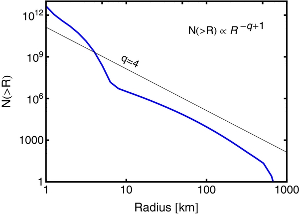
Figure 1. Refer to the following caption and surrounding text. — **Figure 1.** Size distribution at the end of runaway growth before the onset of collisional erosion is given by the thick blue line. Note that during runaway growth, most of the initial mass remains in small planetesimals while a small fraction of the total mass is converted into large protoplanets/KBOs. This specific example corresponds to an initial planetesimal population of bodies that were all 1 km in radius. As shown in Figures 2 and 3, the current large KBO size distribution is well matched by the resulting size distribution from runaway growth. For comparison, a power-law size distribution with differential power-law index q = 4 is given by the thin black line.
Download figure:
Standard image High-resolution image

Figures 2 and 3 show a direct comparison between the results of runaway growth from the coagulation model from Schlichting & Sari (2011) and the observed size distribution of dynamically cold and hot KBOs, respectively. The observed KBO size distribution was derived by Fuentes et al. (2010) by combining results from KBO surveys by Chiang & Brown (1999), Gladman et al. (2001), Trujillo et al. (2001), Allen et al. (2002), Bernstein et al. (2004), Petit et al. (2006), Fraser et al. (2008), Fuentes & Holman (2008), Fuentes et al. (2009, 2010), and Fraser & Kavelaars (2009). Here dynamically cold refers to objects with inclinations less than 5°, whereas dynamically hot corresponds to those with i > 5°. The agreement of the observations with the simple coagulation model from Schlichting & Sari (2011) is good. Figures 2 and 3 show that both the cold and hot populations can be fit by the same size distribution, with the notable difference that the largest bodies in each population grew to different typical sizes.

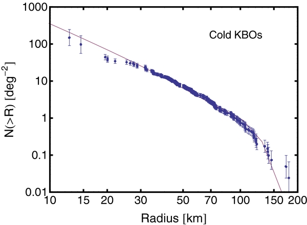
Figure 2. Refer to the following caption and surrounding text. — **Figure 2.** Comparison between the observed Kuiper Belt size distribution for objects with inclinations ⩽5°, also referred to as the cold population, as summarized in Fuentes et al. (2010; points), with the numerical coagulation results from Schlichting & Sari (2011; line). The error bars give the 1σ errors on the cumulative size distribution. The observed Kuiper Belt size distribution above R ∼ 30 km is well matched by planet formation models of runaway growth. Note the break in the size distribution at R ∼ 30 km. We assumed an albedo of 4% and a distance of 42 AU when converting the observed magnitudes into radii. We note here, however, that the exact choice for the value of the albedo does not affect the fit between the observational data and the numerical results because assuming a different value for the albedo would simply shift the x-axis values by a constant and this shift can be matched by the numerical results by letting the self-similar growth continue to larger/smaller sizes.
Download figure:
Standard image High-resolution image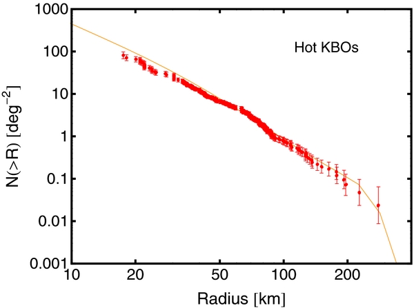

Figure 3. Refer to the following caption and surrounding text. — **Figure 3.** Comparison between the observed Kuiper Belt size distribution for objects with inclinations >5°, also referred to as the hot population, as summarized in Fuentes et al. (2010; points), with the numerical coagulation results from Schlichting & Sari (2011; line). The error bars give the 1σ errors on the cumulative size distribution. The observed Kuiper Belt size distribution above R ∼ 30 km is well matched by planet formation models of runaway growth. Note the break in the size distribution at R ∼ 30 km does not seem as strongly pronounced as in Figure 2.
Download figure:
Standard image High-resolution image

Provided that the fall off at large KBO sizes is not due to some selection effect, this suggests that KBOs grew to typical radii of about 100 km in the cold population and to typical radii of about 300 km in the hot population. If the growth in the hot and cold populations was terminated simultaneously, presumably by the excitation of the velocity dispersion of the growing KBOs and the smaller planetesimals, then this suggests that the hot population may have formed closer to the Sun than the cold population because the shorter orbital periods and likely higher mass surface densities ensure faster growth at smaller semi-major axis.

Observations, including the data plotted in Figures 2 and 3, suggest that there is a break at around 30 km in the KBO size distribution (e.g., Bernstein et al. 2004; Fuentes & Holman 2008; Fraser & Kavelaars 2009; Schlichting et al. 2009; Fuentes et al. 2010). This break is usually attributed to collisional evolution of bodies with R < 30 km over the age of the solar system (e.g., Dohnanyi 1969; Kenyon & Bromley 2004; Pan & Sari 2005). The KBO size distribution below radii of ∼10 km is still poorly constrained because KBOs of these sizes are too small to be detected in reflected light. They can, however, be detected indirectly by stellar occultations. Recent KBO occultation surveys provide the first estimates for the abundance and upper limits of kilometer-sized to sub-kilometer-sized KBOs (e.g., Liu et al. 2008; Schlichting et al. 2009, 2012; Bianco et al. 2010; Zhang et al. 2013).

The work presented in this paper focuses on the size distribution of small KBOs below the break. We model the growth and the subsequent collisional evolution in the Kuiper Belt self-consistently by following the collisional evolution over 4.5 Gyr of the whole KBO size distribution that resulted from runaway growth. We find that the break radius at R ∼ 30 km and size distribution below the break are well matched by collisional evolution models that use published strength laws and make testable predictions for the small KBO size distribution. We show that the excess mass in small planetesimals from the runaway growth phase leaves a permanent signature in the size distribution of small bodies that is not erased after 4.5 Gyr of collisional evolution. Observations of the small KBO size distribution can therefore test if large KBOs grew as a result of runaway growth and constrain the initial planetesimal sizes.

This paper is structured as follows. We describe our Kuiper Belt growth and collisional evolution model in Section 2. In Section 3, we present our results and compare them with current observational constrains on small objects in the Kuiper Belt. Discussion and conclusions follow in Section 4.

2. KUIPER BELT GROWTH AND COLLISIONAL EVOLUTION MODEL

2.1. Growth Model

We use the same coagulation model as described in Schlichting & Sari (2011), which follows the mass growth and the coupled evolution of the velocity dispersion using Safronov's statistical approach (Safronov 1969). We refer the reader to Schlichting & Sari (2011) for the full set of equations for the growth rates of the bodies in the different mass bins and for the corresponding evolution of their velocity dispersions. We investigate the KBO growth in a single annulus centered at 40 AU from the Sun with a width of 10 AU and start the simulations with a total mass of about 20 Earth masses in small planetesimals. This mass surface density was derived by extrapolating the minimum mass solar nebula (Hayashi 1981) to 40 AU after it had been enhanced by a factor of a few as required for the formation of Uranus and Neptune (e.g., Goldreich et al. 2004; Dodson-Robinson & Bodenheimer 2010). We assume that when the relative velocity exceeds the escape velocity of the larger of the two bodies (i.e., $v_{{\rm rel}} > v_{{\rm esc}_{B}}$ ) no accretion occurs and that, if the center of mass collisional energy of two colliding bodies exceeds the catastrophic destruction threshold, fragmentation takes place (see Section 2.2 for details).

In the Kuiper Belt planet formation never went all the way to completion. The growth was likely terminated due to the excitation of the velocity dispersion of the growing KBOs and small planetesimals by the formation and migration of the planets in the outer solar system. We model this dynamical excitation by increasing the velocity dispersion of all bodies in our numerical model to 1 km s⁻¹, which corresponds roughly to the random velocity dispersion in the Kuiper Belt today once objects with the size of Pluto have formed. As long as most of the initial mass resides in planetesimals that are about 1 km in size or larger, destructive collisions and fragmentation are not important until objects comparable to the size of Pluto have formed. This is because initially the planetesimal velocities are smaller than their escape velocities and even as their velocity dispersions are stirred by the growing KBOs, objects of at least several hundreds of kilometers in radius have to form until they can dynamically excite the velocity dispersion of the small planetesimals above speeds needed for destructive collisions.⁵ This picture changes completely once the velocity dispersions of all bodies are excited to 1 km s⁻¹. From this time onward the growth is essentially terminated and destructive collisions lead to the onset of a collisional cascade. We assume, although objects in the hot and cold population likely formed at somewhat different locations, that they evolve together collisionally over the age of the solar system. This assumption is likely valid because the same physical processes, i.e., the formation and migration of Neptune, that are responsible for the excitation of the KBOs' velocity dispersion are responsible for placing the hot population into its current location. The KBO formation timescales are generally found to be less than 100 Myr (e.g., Kenyon & Luu 1999; Schlichting & Sari 2011), which suggests that the Kuiper Belt had close to 4.5 Gyr to evolve collisionally. Observations of the Kuiper Belt size distribution find that the break radius and the slope of the size distribution below the break are the same in both the hot and cold KBO population, which is consistent with the idea that these two populations are undergoing collisional evolution together (Fuentes et al. 2010).

2.2. Collisional Model

We model destructive collisions in the following way. The catastrophic destruction threshold, $Q^*_D$ , is defined as the specific energy needed to disperse the targets into a spectrum of individual objects such that the largest one has exactly half the mass of the original target. When the center of mass collisional energy of two colliding bodies, m₁ and m₂, exceeds the catastrophic destruction threshold, $Q^*_D$ , then the combined mass, m₁ + m₂, is distributed such that one body of mass 0.5(m₁ + m₂) is formed and the remaining mass is distributed as debris over all mass bins that correspond to planetesimal sizes with m < 0.5(m₁ + m₂) according to a differential power-law size distribution given by $dN/dR \propto R^{-q^*}$ .

Since the Kuiper Belt consists of mostly icy bodies with an average velocity dispersion of about 1 km s⁻¹, we adopt the strength law from Leinhardt & Stewart (2009) for ice and 1 km s⁻¹ impact speeds for the catastrophic destruction threshold, which is given by

$\begin{eqnarray} &&Q^*_D=1.3 \times 10^6 \left(\frac{R}{1\ \rm {cm}}\right)^{-0.4}+0.08 \left(\frac{R}{1\ \rm {cm}}\right)^{1.3}\ \rm {erg\ g^{-1}}.\nonumber \\ \end{eqnarray} \tag{ 2 }$

Figure 4 shows $Q^*_D$ as a function of size and the transition from the gravity dominated regime (R ≳ 0.1 km) to the material strength dominated regime (R ≲ 0.1 km). For comparison, the catastrophic destruction threshold corresponding to the specific gravitational binding energy in the gravity regime and the same material strength law as before is also shown in Figure 4. The gravitational binding energy gives an interesting absolute lower limit to the catastrophic destruction threshold, since bodies cannot be weaker than this.

Figure 4. Refer to the following caption and surrounding text. — **Figure 4.** Catastrophic destruction threshold, $Q^*_D$ , as a function of size. The solid blue line corresponds to results from Leinhardt & Stewart (2009) for ice and 1 km s⁻¹ impact velocities, which corresponds to the velocity dispersion in the Kuiper Belt today. For comparison, the catastrophic destruction threshold corresponding to the gravitational binding energy in the gravity regime and the same material strength law as before is shown as the dashed blue line. The gravitational binding energy gives an absolute lower limit to the catastrophic destruction threshold since bodies cannot be weaker than this.
Download figure:
Standard image High-resolution image

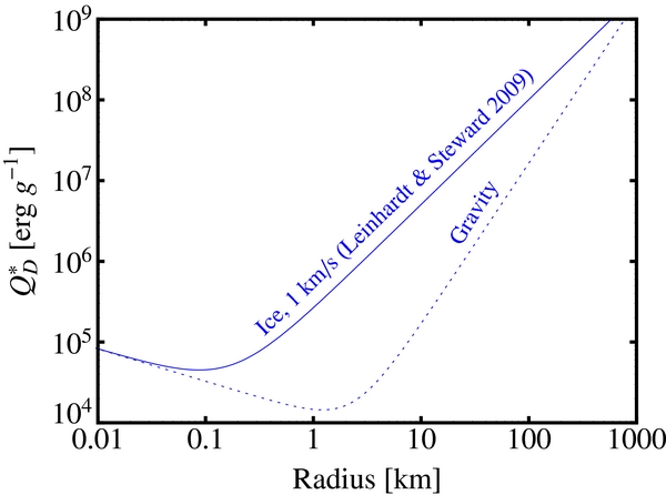
**Figure 4.** Catastrophic destruction threshold, $Q^*_D$ , as a function of size. The solid blue line corresponds to results from Leinhardt & Stewart (2009) for ice and 1 km s⁻¹ impact velocities, which corresponds to the velocity dispersion in the Kuiper Belt today. For comparison, the catastrophic destruction threshold corresponding to the gravitational binding energy in the gravity regime and the same material strength law as before is shown as the dashed blue line. The gravitational binding energy gives an absolute lower limit to the catastrophic destruction threshold since bodies cannot be weaker than this.
Download figure:
Standard image High-resolution image

For the fragment size distribution, $dN/dR \propto R^{-q^*}$ , we adopt q* = 3.68. This value of q* corresponds to the expected collisional equilibrium size distribution, which has a power-law index that is given by

$\begin{equation} q_{{\rm eq}}=\frac{21+\alpha }{6+\alpha }, \end{equation} \tag{ 3 }$

where α is the exponent of R in $Q^*_D$ (see Equation (2)) in the material strength dominated regime (e.g., Pan & Schlichting 2012). From Equation (3) we find that α = −0.4 yields q_eq = 3.68.

3. RESULTS

Combining our growth and collisional model we investigated the evolution of the KBO size distribution starting from various initial planetesimal sizes over 4.5 Gyr.

3.1. 1 km-sized Planetesimals

Figures 5 and 6 show the resulting KBO size distribution (solid blue line) after 4.5 Gyr of growth and collisional evolution when starting from an initial planetesimal size distribution that consists solely of 1 km-sized bodies, and from an initial planetesimal size distribution that has equal mass per logarithmic mass bin for bodies ranging from 0.4 km to 4 km in radius, respectively. For comparison, the dashed blue lines in Figures 5 and 6 show the KBO size distribution at the end of runaway growth just before the start of destructive collisions. First of all, it is interesting to note that the resulting small KBO size distributions do not follow a single power law below the break (i.e., below R ∼ 30 km) as one may naively expect. Instead we find that the small KBO size distribution exhibits a strong deficit of bodies around R ∼ 10 km in size and a strong excess of bodies around 2 km in radius compared to abundances from a single power-law size distribution spanning the range from 0.1 km to 30 km. This deficit and excess are caused by the planetesimal size distribution left over from the runaway growth phase, which left most of the initial mass in small planetesimals. This excess mass in small planetesimals leaves a permanent signature in the size distribution of small bodies that is not erased after 4.5 Gyr of collisional evolution. The resulting KBO size distributions shown in Figures 5 and 6 are both consistent with abundance estimates and upper limits from KBO occultation surveys (Schlichting et al. 2012; Zhang et al. 2013) shown in black. However, if all the mass initially resides solely in 1 km planetesimals, not quite enough mass is depleted in the 10–30 km radius range compared to observations (see Figure 5). If, on the other hand, we start with an initial planetesimal size distribution that has equal mass per logarithmic mass bin for bodies ranging from 0.4 km to 4 km in radius we find good agreement with the observations (see Figure 6).

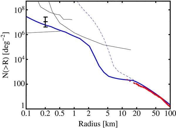
Figure 5. Refer to the following caption and surrounding text. — **Figure 5.** Small KBO size distribution after 4.5 Gyr of collisional evolution for an initial planetesimal population that consisted of 1 km radii objects (blue thick line). For comparison, the KBO size distribution at the end of runaway growth and at the onset of destructive collisions is given by the dashed blue line. The observed KBO size distribution is shown by the red points (Fuentes et al. 2010). The black point with error bars and the thin black lines ranging from 0.1 km to 1 km represent the best estimate and the 95% upper and lower limits on the small KBO population from the *HST*-FGS occultation survey by Schlichting et al. (2012), respectively. The thin black line ranging from 0.2 km to 20 km represents the 95% upper limit on the small KBO population from TAOS (Zhang et al. 2013).
Download figure:
Standard image High-resolution image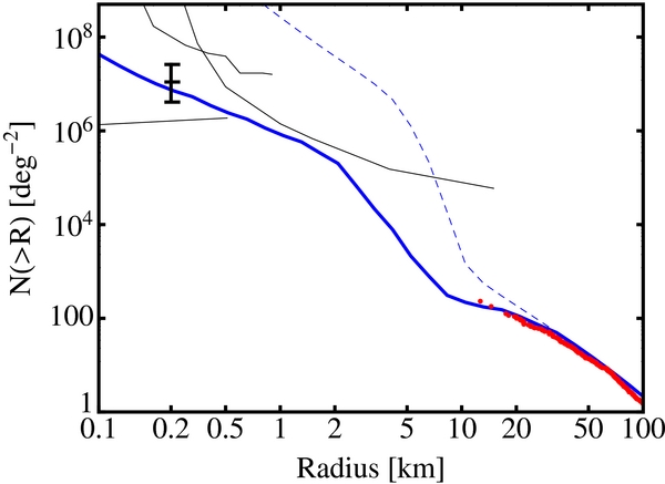

Figure 6. Refer to the following caption and surrounding text. — **Figure 6.** Small KBO size distribution after 4.5 Gyr of collisional evolution for an initial planetesimal population that contained equal mass per logarithmic mass bin in bodies ranging from 0.4 km to 4 km in radius (blue thick line). For comparison, the KBO size distribution at the end of runaway growth and at the onset of destructive collisions is given by the dashed blue line. The observed KBO size distribution is shown by the red points (Fuentes et al. 2010). The black point with error bars and the thin black lines ranging from 0.1 km to 1 km represent the best estimate and the 95% upper and lower limits on the small KBO population from the *HST*-FGS occultation survey by Schlichting et al. (2012), respectively. The thin black line ranging from 0.2 km to 20 km represents the 95% upper limit on the small KBO population from TAOS (Zhang et al. 2013).
Download figure:
Standard image High-resolution image

Figure 7 shows the same collisionally evolved size distribution as in Figure 6 but with the corresponding power-law indices for the different segments. KBOs with R ≳ 30 km follow a size distribution with a differential power-law index q ∼ 4, which is a relic from their formation and has not been modified by collisional evolution over 4.5 Gyr. The power-law index of the size distribution between 0.1 km and 30 km changes from q ∼ 2 (10 km ≲ R ≲ 30 km) to q ∼ 5.8 (2 km ≲ R ≲ 10 km) and then to q ∼ 2.5 (0.1 km ≲ R ≲ 2 km). This change in the slopes of the size distributions is mainly caused by the excess population of planetesimals that was left over from the runaway growth phase. This excess population gives rise to a very steep size distribution between ∼2 km and ∼10 km which grows shallower in time (see Figure 8) because the excess in kilometer-sized planetesimals is being depleted with time. The shallow, q = 2.0, power-law index between ∼10 km and ∼30 km is due to the excess population of kilometer-sized planetesimals that started to deplete the population of bodies between ∼10 km and ∼30 km. The size distribution for R ≲ 0.1 km takes on the expected equilibrium value for material strength dominated bodies as calculated in Section 2.2 from Equation (3) for the catastrophic destruction threshold from Leinhardt & Stewart (2009) for ice and impact velocities of 1 km s⁻¹. The precise values of the power-law index in the different size regimes and the exact location of the inflection points depend on the catastrophic destruction criterion as a function of radius and the initial planetesimal size distribution. For example, starting with planetesimal sizes that range from 0.4 km to 4 km with equal mass per logarithmic mass interval yields a smaller value for q in the 1–10 km range than starting with all the mass in 1 km-sized planetesimals (see Figures 5 and 6 for comparison). However, the overall behavior, i.e., a deficit of bodies around R ∼ 10 km and an excess of bodies around 2 km in radius, does not depend on the exact choices of the catastrophic destruction criterion (i.e., we get similar results if we use strength laws from Benz & Asphaug 1999 instead of the strength laws from Leinhardt & Stewart 2009) and the initial planetesimal size distribution.

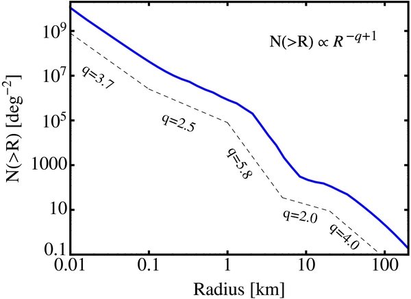
Figure 7. Refer to the following caption and surrounding text. — **Figure 7.** Same small KBO size distribution after 4.5 Gyr of collisional evolution as shown in Figure 6 but plotted with the corresponding differential power-law indices for the different segments of the size distribution. The deficit around 10 km results from an excess of ∼1 km planetesimals at the onset of the collisional evolution. The size distribution for R ≲ 0.1 km takes on the expected equilibrium value for material strength dominated bodies as calculated in Section 2.2. The size distribution above R ∼ 30 km remains unchanged by collisional evolution over the age of the solar system and is therefore primordial.
Download figure:
Standard image High-resolution image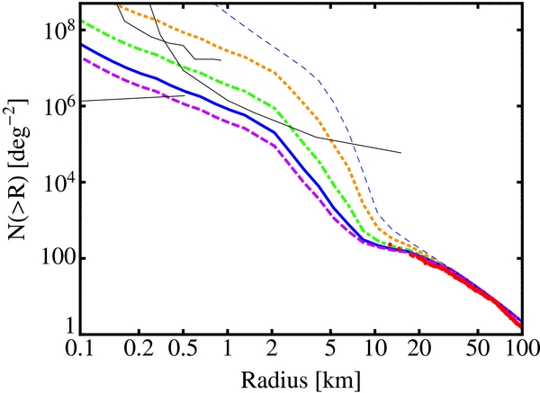

Figure 8. Refer to the following caption and surrounding text. — **Figure 8.** Time evolution of the small KBO size distribution for an initial planetesimal population that contained equal mass per logarithmic mass bin in bodies ranging from 0.4 km to 4 km in radius. The thin blue line corresponds to the KBO size distribution at the end of runaway growth before the onset of destructive collisions; the yellow, dotted line corresponds to 100 Myr; the green dot-dashed line to 1 Gyr; the solid, blue line to 4.5 Gyr; and the dashed purple line to 10 Gyr of collisional evolution. The observed KBO size distribution is shown by the red points (Fuentes et al. 2010). The thin black lines ranging from 0.1 km to 1 km represent the 95% upper and lower limits on the small KBO population from the *HST*-FGS occultation survey by Schlichting et al. (2012) and the thin black line ranging from 0.2 km to 20 km represents the 95% upper limit on the small KBO population from TAOS (Zhang et al. 2013).
Download figure:
Standard image High-resolution image

Figure 8 displays the time evolution of the small KBO size distribution. The differential power-law indices between ∼10 km and ∼30 km and between ∼2 km and ∼10 km become shallower with time. The decrease in the power-law index between ∼2 km and ∼10 km is due to the fact that the excess population of planetesimals that was left over from the runaway growth, which gave rise to a very steep size distribution between ∼2 km and ∼10 km (dashed blue line in Figure 8), is being depleted by destructive collisions with time. The decrease in the power-law index between ∼10 km and ∼30 km is due to the excess population of kilometer-sized planetesimals that start to deplete the population of bodies between ∼10 km and ∼30 km, i.e., the catastrophic destruction threshold from Leinhardt & Stewart (2009) yields, for a velocity dispersion of 1 km s⁻¹, that 10 km-sized bodies are typically destroyed by bodies ∼1 km in radius and 30 km-sized bodies are typically destroyed by bodies that are ∼8 km in radius. The power-law index below ∼2 km evolves to q ∼ 2.5 and remains close to constant from then onward.

3.2. 10 km-sized Planetesimals

Figure 9 shows the resulting small KBO size distribution after 4.5 Gyr of collisional evolution for an initial planetesimal population that consisted of 10 km radius bodies (solid blue line). The small KBO size distribution is inconsistent with the observed size distribution of KBOs with radii ranging from 10 km to 100 km (red points) and with upper limits from the TAOS KBO occultation survey (Zhang et al. 2013). Even if we assume that large KBOs are only held together by their own gravity (blue dotted line in Figure 9), which is an absolute lower limit on their strength, because bodies cannot be weaker than this, we find that we cannot match the observed KBO size distribution. We also started with initial planetesimal populations that contained equal mass per logarithmic mass interval between 1 km and 10 km in radius and were still unable to find a reasonable agreement between the resulting small KBO size distribution and the observations. This leads us to conclude that the Kuiper Belt did not form via coagulation from an initial planetesimal population that contained most of the initial mass in planetesimals that were 10 km in radius or larger, because not enough of the initial planetesimals can be ground down over the age of the solar system to match observations. These findings are in agreement with similar results obtained for the asteroid belt by Weidenschilling (2011), for debris disks by Kenyon & Bromley (2010) and for the outer solar system by Kenyon & Bromley (2012), which all point to initial planetesimal sizes that are less, maybe much less, than 10 km in radius.

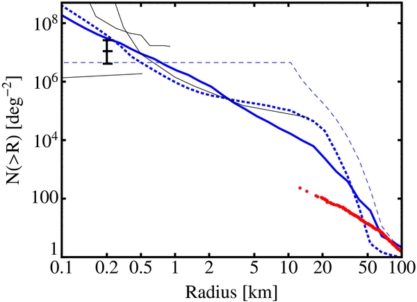
Figure 9. Refer to the following caption and surrounding text. — **Figure 9.** Small KBO size distribution after 4.5 Gyr of collisional evolution for an initial planetesimal population that consisted of 10 km radius bodies (blue thick line). The resulting size distribution assuming that large KBOs are solely held together by their own gravity is shown by the dotted blue line. For comparison, the KBO size distribution at the end of runaway growth and at the onset of destructive collisions is given by the dashed blue line. The observed KBO size distribution is shown by the red points. The black point with error bars and the thin black lines ranging from 0.1 km to 1 km represent the best estimate and the 95% upper and lower limits on the small KBO population from the *HST*-FGS occultation survey by Schlichting et al. (2012), respectively. The thin black line ranging from 0.2 km to 20 km represent the 95% upper limit on the small KBO population from TAOS (Zhang et al. 2013). The resulting KBO size distributions are inconsistent with the observed KBO size distribution for bodies with radii ranging from 10 km to 100 km and with upper limits from the TAOS KBO occultation survey (Zhang et al. 2013). This result holds true even if we assume that large KBOs are only held together by their own gravity. We conclude that the Kuiper Belt did not form from 10 km-sized planetesimals by coagulation, because not enough of the initial planetesimals can be ground down over the age of the solar system to match observations.
Download figure:
Standard image High-resolution image

4. DISCUSSION AND CONCLUSIONS

We studied the size distribution of small KBOs by modeling self-consistently the growth and the subsequent collisional evolution over 4.5 Gyr in the Kuiper Belt and arrive at the following results.

1.
The Kuiper Belt size distributions of the cold and hot population for radii ≳ 30 km are primordial and both can be well fit by the resulting size distributions from planet formation models of runaway growth (see Figures 2 and 3) with the notable difference that the largest bodies in the hot population grew to larger radii than in the cold population, which is consistent with the idea that the hot population formed at a smaller semi-major axis compared to the cold population.
2.
The break radius at R ∼ 30 km and size distribution below the break are well matched by collisional evolution models that use published strength laws (Leinhardt & Stewart 2009) and start with resulting size distributions from runaway growth and follow the collisional evolution in the Kuiper Belt over 4.5 Gyr. This suggests that the Kuiper Belt may indeed be the solar system analog of the dust-producing debris disks observed around other stars (e.g., Backman & Paresce 1993; Carpenter et al. 2009; Kenyon & Bromley 2010; Kennedy & Wyatt 2010).
3.
Compared to a single power-law size distribution that would span the whole range from 0.01 km to 30 km, we find in general a strong deficit of bodies around R ∼ 10 km and a strong excess of bodies around 2 km in radius. This deficit and excess are caused by the planetesimal size distribution left over from the runaway growth phase, which leaves most of the initial mass in small bodies. This excess mass in small planetesimals leaves a permanent signature in the size distribution of small bodies that is not erased after 4.5 Gyr of collisional evolution. Future KBO occultation surveys, which probe the small KBO size distribution, can therefore test if large KBOs grew as a result of runaway growth and constrain the initial planetesimal sizes.
4.
The observed KBO size distribution derived by Fuentes et al. (2010) by combining various KBO surveys (Chiang & Brown 1999; Gladman et al. 2001; Trujillo et al. 2001; Allen et al. 2002; Bernstein et al. 2004; Petit et al. 2006; Fraser et al. 2008; Fuentes & Holman 2008; Fuentes et al. 2009, 2010; Fraser & Kavelaars 2009) and results from recent optical KBO occultation surveys (Schlichting et al. 2012; Zhang et al. 2013) are best matched by an initial planetesimal population that contained about equal mass in bodies ranging from 0.4 km to 4 km in radius. In addition, the resulting KBO size distribution after 4.5 Gyr of collisional evolution is also consistent with upper limits from KBO occultation surveys at X-ray wavelengths that probe objects ranging from ∼30 m to 300 m in radius (Jones et al. 2008; Chang et al. 2011, 2013).
5.
The observed KBO size distribution for R > 10 km cannot be matched if most of the initial planetesimal mass resided in bodies that were 10 km in radius or larger, because their resulting size distribution cannot be sufficiently depleted over 4.5 Gyr to match observations. We conclude from this that the Kuiper Belt did not form by coagulation from an initial planetesimal size distribution that contained most of its mass in planetesimals with radii of 10 km or larger. These results are in agreement with similar findings obtained for the asteroid belt by Weidenschilling (2011) and for debris disks by Kenyon & Bromley (2010), which both point to small initial planetesimal sizes with R ≲ 100 m and R ≲ 10 km, respectively.

There are several further interesting things to note here.

Since the excess mass in small planetesimals from the runaway growth phase leaves a permanent signature in the size distribution of small bodies that is not erased after 4.5 Gyr of collisional evolution, future KBO occultation surveys will be able to test whether large KBOs grew as a result of runaway growth from an initial planetesimal population consisting of bodies ranging from a few hundred meters to a few kilometers in size. The small KBO size distribution therefore offers the opportunity to observationally constrain the initial planetesimal sizes from which planets form, which remains one of the major open questions in planet formation theory (Chiang & Youdin 2010).

The resulting small KBO size distributions that we find all contain enough bodies to satisfy the required supply rate for the Jupiter family comets (Volk & Malhotra 2008). If the Kuiper Belt formed by coagulation from kilometer-sized planetesimals then there should be an excess of about a factor of 1000 of small comets with initial radii (i.e., before any mass loss or break up occurs) of 2 km compared to 10 km.

Because the comet size distribution has likely been modified by mass loss and break up of the cometary nuclei, the size distribution of centaurs should provide a more reliable probe of the KBO size distribution between 1 and 10 km in radius. Unfortunately, although about two hundred centaurs are currently known with sizes ranging from about 100 km to 1 km, no well characterized survey has been carried out to date that would allow the derivation of a de-biased centaur size distribution and therefore probe the small KBO size distribution.

Finally, it is very intriguing that there is a striking similarity between the small KBO size distribution that we find after 4.5 Gyr of collisional evolution and the reconstructed impact size distribution from the cratering records on the Saturnian satellites (Minton et al. 2012). Minton et al. (2012) find that the cratering size distribution of the old terrains of Dione, Hyperion, Iapetus, Mimas, Phoebe, Rhea, and Tethys can be explained by a single impactor population that follows a size distribution with differential power-law indices of q = 4 for R > 30 km, q = 2.0 for 10 km < R < 30 km, q = 4.2 for 1 km < R < 10 km, q = 2.6 for 0.1 km < R < 1 km, and q = 3.7 for 0.01 km < R < 0.1 km. These values are in remarkably good agreement with the power-law indices that we find for the small KBO size distribution and which are shown in Figure 7. The only notable difference between our small KBO size distribution and the results from Minton et al. (2012) seems to be in the range from ∼1 km to ∼10 km for which we find a steeper size distribution with power-law index q = 5.8. The similarities between our results for the small KBO size distribution and the reconstructed impactor size distribution suggest that the impactors that bombarded the Saturnian moons originated from the Kuiper Belt.

We thank David Jewitt for his comments and suggestions and are grateful for constructive comments and suggestions from the referee. For H.S., support for this work was provided by NASA through Hubble Fellowship Grant No. HST-HF-51281.01-A awarded by the Space Telescope Science Institute, which is operated by the Association of Universities for Research in Astronomy, Inc., for NASA, under contact NAS 5-26555.

INITIAL PLANETESIMAL SIZES AND THE SIZE DISTRIBUTION OF SMALL KUIPER BELT OBJECTS

Authors

Author notes

Notes

Article metrics

Permissions

Share this article

Article information

Dates

ABSTRACT

Related links