
Abstract
SDSS-IV MaNGA (Mapping Nearby Galaxies at Apache Point Observatory) is the largest integral-field unit (IFU) spectroscopy survey to date, aiming to observe a statistically representative sample of 10,000 low-redshift galaxies. In this paper, we study the reliability of the emission-line fluxes and kinematic properties derived by the MaNGA Data Analysis Pipeline (DAP). We describe the algorithmic choices made in the DAP with regards to measuring emission-line properties, and the effect of our adopted strategy of simultaneously fitting the continuum and line emission. The effects of random errors are quantified by studying various fit-quality metrics, idealized recovery simulations, and repeat observations. This analysis demonstrates that the emission lines are well fit in the vast majority of the MaNGA data set and the derived fluxes and errors are statistically robust. The systematic uncertainty on emission-line properties introduced by the choice of continuum templates is also discussed. In particular, we test the effect of using different stellar libraries and simple stellar-population models on the derived emission-line fluxes and the effect of introducing different tying prescriptions for the emission-line kinematics. We show that these effects can generate large (>0.2 dex) discrepancies at low signal-to-noise ratio and for lines with low equivalent width (EW); however, the combined effect is noticeable even for Hα EW > 6 Å. We provide suggestions for optimal use of the data provided by SDSS data release 15 and propose refinements on the DAP for future MaNGA data releases.
1. Introduction
Advances in our understanding of galaxy evolution are fundamentally linked to the development of increasingly sophisticated models to derive physical properties from observables. Integral-field spectroscopy (IFS) surveys of nearby galaxies, combining large-number statistics with the information content of resolved spectroscopy, represent some of the richest data sets currently available to the astronomical community and pose their own specific data-modeling challenges. Modern IFS surveys of nearby galaxies—including ATLAS3D (Cappellari et al. 2011), CALIFA (Sánchez et al. 2012), SAMI (Croom et al. 2012), and MaNGA (Bundy et al. 2015)—are designed around a wide variety of science goals, which often rely on the simultaneous determination of the stellar and gas kinematics, emission-line ratios, and stellar-population properties (like age and metallicity) via specialized tools.
To provide users with readily available model-independent high-level data products, the SDSS-IV (Sloan Digital Sky Survey) MaNGA survey has developed a data analysis pipeline (DAP) to process the reduced MaNGA datacubes in an automated and uniform way, which has now been released publicly for the first time. In addition to fully reduced data products, the 15th SDSS Data Release (DR15; Aguado et al. 2019) includes the output of the MaNGA DAP for an unprecedented sample of 4688 spatially resolved galaxies.
A detailed description of the DAP design workflow and output is presented in Westfall et al. (2019). In short, the MaNGA DAP is a project-led software effort designed to be both an automated pipeline and a general-purpose tool. For DR15, the DAP provides stellar kinematics, emission-line properties, and assessments of stellar-continuum features as measured by spectral indices, such as the Lick indices and D4000.
Westfall et al. (2019) present a detailed assessment of the stellar kinematics provided by the DAP. Here we provide a complementary analysis of the emission-line properties, focusing on fluxes and kinematics. We validate the measurements as well as the statistical fidelity of the DAP-produced uncertainties. Our approach follows both the classical perspective of adding noise to mock data as well as making use of repeat observations specifically obtained for testing the repeatability of the MaNGA survey output.
Importantly, we also recognize that the derivation of emission-line fluxes and kinematics suffers from a certain amount of model-dependent systematics. In this work, therefore, we explore several sources of systematic error—for example, the use of different stellar-continuum templates, how one ties the kinematic parameters of different emission lines, and the simultaneous or sequential optimization of fits of the emission lines and underlying continuum. Although these issues are not new to the literature, we discuss them here in a coherent framework, which we hope will constitute a useful reference for the spectral-fitting community beyond the users of the MaNGA data set itself.
A key aspect of accurately measuring the nebular emission lines is properly accounting for the stellar continuum. This is particularly important for the Balmer lines, where underlying stellar absorption can reduce the Hβ emission-line equivalent width (EW) by up to 10 Å at low spectral resolution (Groves et al. 2012). In early work focused on H ii regions, it was common to assume a constant 2 Å correction (McCall et al. 1985). The development of more sophisticated stellar-population models enabled a more rigorous approach whereby the stellar continuum is fit using a linear combination of simple stellar-population models (SSPs) with reddening treated as an additional free parameter. This approach was first applied on a large scale to the SDSS data by the MPA-JHU group in their analysis of the SDSS-I spectra (Brinchmann et al. 2004; Tremonti et al. 2004; Aihara et al. 2011). They carried out the fitting in two stages: first, they masked the emission lines and modeled the stellar continuum using a linear combination of Bruzual & Charlot (2003) SSP models modified by a Charlot & Fall (2000) dust law with the velocity dispersion and redshift constrained a priori. Next, the stellar continuum was subtracted, low-order residuals were removed using a sliding median, and the emission lines were simultaneously fit with Gaussian functions.
A downside of treating the stellar-population modeling and emission-line fitting as separate steps is that valuable regions of the spectrum are masked during the continuum fit and uncertainties in the continuum fit are not propagated forward into the emission-line fits. To circumvent these issues and accurately measure very weak lines in early-type galaxies, Sarzi et al. (2006) introduced a routine called GANDALF (gas and absorption-line fitting algorithm), based on an early version of pPXF (Cappellari & Emsellem 2004), that simultaneously fits the stellar continuum and nebular emission lines, given a previously determined stellar kinematics solution for the continuum. This code was subsequently applied to the SDSS data by Oh et al. (2011).
IFS data pose a particular challenge to analyze because the outer regions of galaxies often have low signal-to-noise ratio (S/N) in the continuum (i.e., S/N per pixel of 3–5). This makes it difficult to accurately constrain the stellar continuum, especially when stellar kinematics are determined simultaneously with stellar-population ages and metallicities. The penalized pixel-fitting (pPXF) software (Cappellari & Emsellem 2004; Cappellari 2017), developed for use on the SAURON data (Emsellem et al. 2004), pioneered a robust pixel-fitting method, particularly optimized for determining template mixes and robust kinematics from data with moderate S/N (∼10–20) and resolution. This technique can be coupled with adaptive Voronoi binning (Cappellari & Copin 2003) to achieve the S/N needed to accurately fit the stellar continuum in IFS data.
The CALIFA survey has led the way in terms of the development of spectral-fitting pipelines suitable for a wide range of galaxy types (e.g., Cid Fernandes et al. 2013). The FIT3D pipeline (Sánchez 2006) and its newer implementation Pipe3D (Sánchez et al. 2016a) have developed a detailed procedure for employing different binning schemes for the stellar and emission-line properties. For example, Pipe3D performs an initial spatial binning based on continuum S/N and analyzes the binned spectra to determine the properties of the stellar continuum. It then rescales the best-fit continuum model to match the flux in each individual spaxel in the bin, subtracts the rescaled continuum, and fits the nebular lines (Sánchez et al. 2016b). An emission-line-free spectrum is then created, and the process is iterated without the emission-line masks.
Other emission-line fitting codes have been developed to optimize the information extracted from different data sets. For example, the SAMI IFS data set has higher spectral resolution in its red-wavelength arm than either MaNGA or CALIFA, and, as a consequence, many of the emission lines show complex line profiles that are not well fit by a single Gaussian profile (Hampton et al. 2017; Green et al. 2018). The LZIFU (Ho et al. 2016) code constrains the stellar continuum in individual spaxels using pPXF, and then it fits the emission lines with multiple Gaussians where needed.
In the MaNGA DAP, we employ a “hybrid” binning scheme (Voronoi for the continuum and individual spaxels for the emission lines; see Section 2.2) and simultaneously fit the continuum and emission lines, which is made possible by the latest version (>6.0 in python) of the pPXF software package (Cappellari 2017).15
Although the DAP fits the stellar continuum with the aim of deriving accurate emission-line fluxes, the code does not provide stellar-population properties (age, metallicity, etc.), because the MaNGA team considered these quantities to be too model-dependent to be provided by a general-purpose tool. Stellar population analyses of MaNGA galaxies presented in DR15 are therefore released as value-added catalogs (VACs). In the context of SDSS, a VAC is a product that is not generated by the SDSS project team, but instead contributed by specific members of the collaboration.
Two teams have released catalogs of stellar population properties for the MaNGA galaxies in DR15, constituting the FIREFLY and Pipe3D VACs. FIREFLY (Wilkinson et al. 2015, 2017) is a specialized full-spectral fitting code, which uses the output from the DAP for binning, determination of the stellar kinematics, and subtraction of nebular line emission, and it computes stellar population properties (mean age, metallicity, and dust extinction).
The MaNGA data have been independently analyzed with the Pipe3D (Sánchez et al. 2016a, 2016b) code. Unlike FIREFLY, Pipe3D performs independent measurements of the stellar kinematics and emission lines, in addition to providing stellar population properties. A brief overview of these two VACs can be found in Aguado et al. (2019).
Finally, we warn the potential user that the DAP remains limited in how well suited its output is to certain emission-line-related science goals. For example, studies of chemical composition of the interstellar medium (ISM) within galaxies (Sánchez et al. 2014; Barrera-Ballesteros et al. 2017; Belfiore et al. 2017; Poetrodjojo et al. 2018) rely on accurate derivation of emission-line fluxes and their ratios within H ii regions, and such studies benefit from the highest spatial resolution allowed by the data to avoid contamination from the diffuse ISM. The study of the ISM in early-type galaxies (Sarzi et al. 2010; Belfiore et al. 2016), on the other hand, requires careful modeling of the stellar continuum in order to recover the fluxes of faint low-equivalent-width lines and may benefit from ad hoc spatial binning. Studies of the diffuse ionized ISM (Zhang et al. 2017) and extraplanar gas (Jones et al. 2017) also crucially rely on binning and stacking of low-surface-brightness emission, while galactic outflows can be dissected by careful analysis of asymmetries in the emission-line profiles (Gallagher et al. 2019). We anticipate that several users will use the DAP output as a reference and starting point for more complex and tailored analysis.
In this paper, we describe the algorithmic choices made in the DAP with regards to measuring emission-line properties (Section 2). The effects of random errors are quantified by studying various fit-quality metrics, idealized recovery simulations, and repeat observations in Section 3. The systematic uncertainty in emission-line properties introduced by the choice of continuum templates is analyzed in Section 4. In particular, we test the effect of using different stellar libraries and simple stellar-population models on the derived emission-line fluxes. In Section 5 we consider other systematics introduced by our algorithmic choices, such as the adopted strategy of simultaneously fitting the continuum with the emission lines. In Section 6 we summarize our recommendations for optimal use of the data provided by DR15 and some ideas for future DAP development. A brief summary is given in Section 7. Throughout this paper, and in all data released by SDSS, wavelengths are given in vacuum.
2. The MaNGA DAP Algorithm
2.1. The Input MaNGA Data
The MaNGA survey is one of the three key components of SDSS-IV (Blanton et al. 2017) and aims to obtain IFS data for a representative sample of 10,000 galaxies in the redshift range 0.01 < z < 0.15 by 2020. The MaNGA instrument operates on the SDSS 2.5 m telescope at Apache Point Observatory (Gunn et al. 2006) and consists of a set of 17 hexagonal fiber bundles of different sizes, plus a set of minibundles and sky fibers used for flux calibration and sky subtraction, respectively (Drory et al. 2015; Law et al. 2015; Yan et al. 2016a, 2016b). All fibers are fed into the dual-beam BOSS spectrographs covering the wavelength range from 3600 to 10300 Å with a spectral resolution R ∼ 2000 (Smee et al. 2013).
MaNGA galaxies are selected from an extended version of the NASA-Sloan Atlas (NSA) and are observed out to 1.5 Re (primary sample, comprising two-thirds of the total sample) or 2.5 Re (secondary sample, comprising one-third of the total sample). Targets are selected to be representative of the overall galaxy population at each stellar mass in the range  . In practice, the absolute i-band magnitude is used for sample selection to avoid the systematic uncertainty intrinsic in deriving stellar masses (Wake et al. 2017).
The starting point of this paper is the datacubes produced for DR15 by the MaNGA data-reduction pipeline (DRP; Law et al. 2016), with additional modifications described in Aguado et al. (2019). The MaNGA DAP takes as input the reduced MaNGA datacubes generated with logarithmic wavelength sampling.
An overview of the DAP workflow is presented in Westfall et al. (2019). Here, we summarize the aspects of the algorithm that are most relevant to the derivation of emission-line properties, in order to motivate the tests performed in the rest of the paper. A graphical overview of the relevant components of the DAP workflow is presented in Figure 1 and discussed in the following sections.
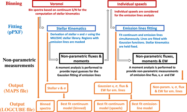
Figure 1. Graphical representation of the DAP workflow. The figure highlights the interplay between different binning schemes (red), fitting steps performed with pPXF (blue), nonparametric measurements (black), and output quantities (orange). The algorithm can be roughly divided into two sections: the first step is dedicated to the extraction of the stellar kinematics (left side of the figure), while the second one performs the simultaneous fitting of gas and stars (right side of the figure). The main outputs produced by the DAP are the MAPS and LOGCUBE files, containing respectively the 2D maps of derived parameters (e.g., velocities, fluxes) and the 3D best-fit models (in datacube format).
Download figure:
Standard image High-resolution image2.2. Overview of the MaNGA DAP with Regards to Emission Lines
The DAP currently performs two full-spectrum fits, both using pPXF. The first fit primarily determines the stellar kinematics, and the second models the emission lines. Two example spectra fitted by the MaNGA DAP can be inspected in Figure 2. For DR15, the stellar kinematics are determined only for spectra binned to g-band S/N > 10, as produced by applying the Voronoi binning algorithm implemented in the python language16 by Cappellari & Copin (2003). The subsequent emission-line modeling is done for both the binned spectra and after deconstructing the bins into the individual spaxels; a full description of the emission-line-fitting module of the DAP is provided in Section 8 of Westfall et al. (2019). Because it is most relevant to emission-line science, we focus on the results provided by the latter approach, which we term the “hybrid” binning scheme (see below).
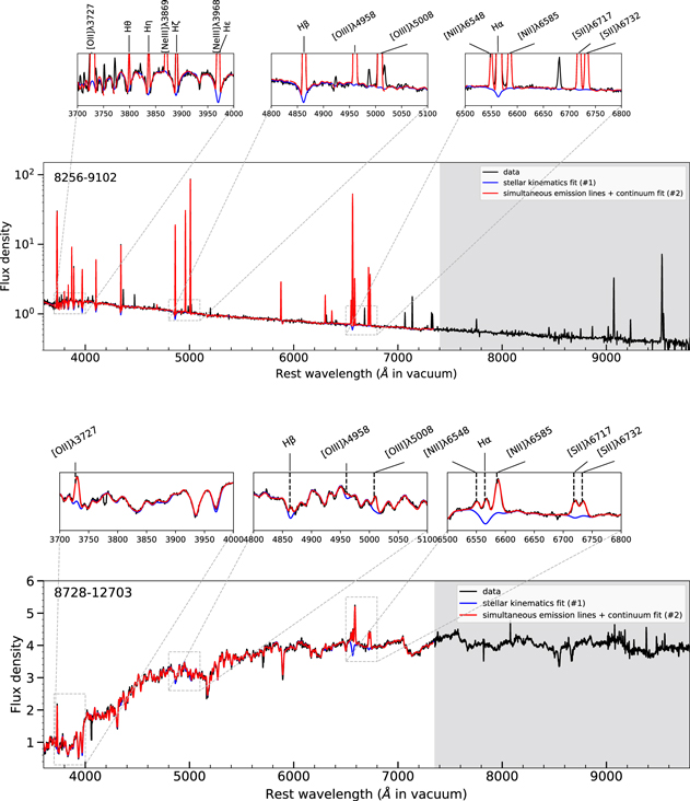
Figure 2. Two spectra fitted by the MaNGA DAP. The top spectrum belongs to the central regions of a star-forming galaxy with very bright emission lines (8256–9102), while the bottom spectrum is taken from the central regions of an early-type galaxy with low-EW line emission (8728–12703). Zoomed-in views are provided for the wavelength regions around [O ii]λλ 3727,29 and the 4000 Å break, Hβ and [O iii]λ5007, and Hα and [N ii]λλ 6548,84. The figures show the data in black, the results of the first fit (optimized for the determination of stellar kinematics) in blue, and the second fit (optimized for emission-line parameters) in red. During the first fit, the spectrum is masked around the expected positions of the main emission lines. The region redder than ∼7400 Å is not fitted in DR15 because of the limited wavelength coverage of the MILES-HC templates.
Download figure:
Standard image High-resolution image2.2.1. Stellar-kinematics Fit (First Fitting Stage)
When using pPXF to determine the stellar kinematics (Westfall et al. 2019, Section 7), spectral regions potentially affected by line emission are masked. The adopted masks extend ±750 km s−1 around the expected emission-line wavelength at the galaxy systemic redshift. In DR15, we use a set of templates determined using a hierarchical-clustering analysis of the MILES stellar library (Sanchez-Blazquez et al. 2006; Falcón-Barroso et al. 2011), which we refer to as the MILES-HC library (see Section 5 of Westfall et al. 2019 and Section 4.1 below). We also include an eighth-order additive Legendre polynomial, motivated by the experience from the SAURON (Emsellem et al. 2004) and ATLAS3D (Cappellari et al. 2011) teams, to improve the quality of the derived kinematics by providing a closer match between data and spectral templates. However, it is important to note that the additive polynomials modify the absorption-line depth of the stellar templates, which becomes important to our discussion in Section 5.2.
2.2.2. Hybrid Binning Approach
Since the line emission surface brightness can be very different from the continuum surface brightness, the relevant binning scale is not necessarily the same for continuum and emission-line science. Indeed, the emission-line fitting can be performed by optimally rebinning the data for the extraction of the emission-line properties (Cid Fernandes et al. 2013; Belfiore et al. 2016; Sánchez et al. 2016b); however, this strategy has not yet been implemented within the DAP. Instead, we model the emission lines in each spaxel as follows: we first remap the best-fitting stellar kinematics determined for the binned spectra to the individual spaxels, and then, keeping the stellar kinematics fixed, we simultaneously optimize the stellar-continuum and emission-line templates to determine the best-fit model spectrum. We refer to this as the “hybrid” binning approach because the stellar kinematics uses the Voronoi-binned data, whereas the emission-line results are for individual spaxels. Importantly, during the emission-line modeling, the algorithm reoptimizes the continuum templates to fit each spaxel, rather than simply rescaling the best-fit stellar continuum from the Voronoi-binned fit to each spaxel (as done, for example, by Pipe3D). The output of this scheme (HYB10-GAU-MILESHC; see below) is the recommended data product in DR15 for users interested in emission-line properties of MaNGA galaxies. A fit to the emission lines on the same Voronoi bins as the stellar continuum is also provided for users whose science goals require, for example, the stellar and gas kinematics to be computed over the exact same spatial scales.
We considered it important in the hybrid binning scheme to fix the stellar kinematics based on the binned spectra when fitting the individual spaxels because nonlinear parameters (such as velocity and σ) may suffer from biases when derived in low-S/N single-spaxel spectra.
2.2.3. Simultaneous Fit of Gas and Stars (Second Fitting Stage)
To simultaneously optimize the fit to the stellar continuum and the emission lines, we use pPXF with Gaussian emission-line templates associated to kinematic parameters that are independent of those used for the stellar templates (Cappellari 2017). Simultaneous fits of emission-line and continuum templates have been introduced and recommended in previous work (Sarzi et al. 2006; Oh et al. 2011) as a way to minimize the bias resulting from masking of the wings of the Balmer absorption profiles and other stellar features on the recovered emission-line fluxes. This approach allows one to enforce the physical constraint that emission lines cannot be negative, while optimizing the fit to the stellar continuum. pPXF adopted the same idea for the gas fitting, but implemented this strategy in a different way, as described in Cappellari (2017). An example of the results of this fitting algorithm can be seen in Figure 2 for both a highly star-forming and an early-type galaxy. We assess the difference in the best-fit models derived by simultaneous versus subsequent fitting of the emission lines in Section 5.1.
The 22 emission lines fit by the DAP in DR15 are presented in Table 1. The flux ratios of doublets are fixed when such ratios are determined by atomic physics (Table 1; Osterbrock & Ferland 2006). For DR15 we tie the velocity of all the fitted emission lines, but do not tie the velocity dispersions with the exception of most of the doublets. Specifically, the line doublets with fixed flux ratios and the [O ii]λλ 3727,29 doublet have their velocity dispersions tied between the doublet lines, but each doublet and all other lines have independent velocity dispersions.17 While tying the kinematics of different emission lines may prove advantageous in recovering the flux of weak lines, we do not tie all velocity dispersions in DR15 to allow for modest inaccuracies (generally a few percent) in the wavelength-dependent line-spread function (LSF) determined by the MaNGA DRP; further discussion of the current line-tying strategy is presented in Section 5.2. Given the limited spectral range of the adopted MILES-HC stellar library, lines redder than ∼7400 Å are not fit for DR15. In future data releases, however, we plan to use templates with a larger wavelength range to allow for a determination of the continuum under the emission lines redder than 7400 Å (see Section 4).
Table 1. Wavelengths and Ionization Potential of the Relevant Ion for Each Emission Line Fit for DR15, Subdivided into the Groups Defined to Study the Different Tying Schemes Described in Section 5.3
| Line Name | Wavelength (Vacuum) (Å) | DAP String Name | Ionization Potential (eV) | Fixed Ratio |
|---|---|---|---|---|
| Hydrogen Balmer Lines | ||||
| Hθ (H10) | 3798.983 | Hthe-3798 | 13.60 | no |
| Hη (H9) | 3836.479 | Heta-3836 | 13.60 | no |
| Hζ (H8) | 3890.158 | Hzet-3890 | 13.60 | no |
| H |
3971.202 | Heps-3971 | 13.60 | no |
| Hδ | 4102.899 | Hdel-4102 | 13.60 | no |
| Hγ | 4341.691 | Hgam-4341 | 13.60 | no |
| Hβ | 4862.691 | Hb-4862 | 13.60 | no |
| Hα | 6564.632 | Ha-6564 | 13.60 | no |
| Low-ionization lines | ||||
| [O ii]λ3727 | 3727.092 | OII-3727 | 13.61 | no |
| [O ii]λ3729 | 3729.875 | OII-3729 | 13.61 | no |
| [O i]λ6300 | 6302.04 | OI-6302 | 0.0 | no |
| [O i]λ6364 | 6365.535 | OI-6365 | 0.0 | 0.328 [O i]λ6300 |
| [N ii]λ6548 | 6549.86 | NII-6549 | 14.53 | 0.327 [N ii]λ6584 |
| [N ii]λ6584 | 6585.271 | NII-6585 | 14.53 | no |
| [S ii]λ6717 | 6718.294 | SII-6718 | 10.36 | no |
| [S ii]λ6731 | 6732.674 | SII-6732 | 10.36 | no |
| High-ionization lines | ||||
| [Ne iii]λ3869 | 3869.86 | NeIII-3869 | 40.96 | no |
| [Ne iii]λ3968 | 3968.59 | NeIII-3968 | 40.96 | no |
| He iiλ4687 | 4687.015 | HeII-4687 | 54.41 | no |
| [O iii]λ4959 | 4960.295 | OIII-4960 | 35.12 | 0.340 [O iii]λ5007 |
| [O iii]λ5007 | 5008.240 | OIII-5008 | 35.12 | no |
| He iλ5876 | 5877.243 | HeI-5877 | 24.58 | no |
Note. Ritz wavelengths in vacuum are taken from the National Institute of Standards and Technology (NIST; http://physics.nist.gov/PhysRefData/ASD/Html/help.html). The DAP string name is reported in the header of the MAPS files for the emission-line extensions and allows the users to associate each map with the correct line (see Section 6.1). Ionization potentials are taken from Draine (2011). Lines redder than ∼7400 Å, corresponding to the red cutoff of the MILES-HC stellar templates, are not fit in DR15.
Download table as: ASCIITypeset image
During the fitting procedure, the DAP does not constrain the emission-line fluxes to follow a specific attenuation law resulting from dust present in the host galaxy (as generally done in GANDALF, e.g., Oh et al. 2011, and optionally available in pPXF). All line fluxes are, however, corrected for Galactic foreground extinction using the maps of Schlegel et al. (1998) and the reddening law of O’Donnell (1994). Users comparing the DAP output with the output generated by other spectral-fitting pipelines may need to take this factor into account.
An eighth-order multiplicative Legendre polynomial is used in DR15 to match the overall spectral shape of the data, which can deviate from that of the models both because of dust extinction and small inaccuracies in the spectrophotometric calibration. A physically motivated extinction law may be used in the MaNGA DAP instead of multiplicative polynomials, but this was found to produce worse fits to the stellar continuum, especially at the blue end of the spectrum (see Section 5.1). Additive polynomials are not, and indeed ought not be, used in this stage as they modify the depth of stellar absorption lines in the templates, therefore potentially leading to degeneracies with emission-line strengths. This point is further elucidated in Section 5.1. Neither polynomials nor extinction corrections are applied to the emission-line templates by the fit, but only to the stellar continuum.
2.2.4. Nonparametric Emission-line Properties and EW
The DAP also calculates nonparametric emission-line moments (zeroth, first, and second), both before and after the emission-line modeling (see Figure 1). Both iterations subtract a best-fit stellar-continuum model before calculating the moments; additional detail is provided in Section 9 and Table 2 of Westfall et al. (2019). The first iteration subtracts the best-fit stellar continuum used to determine the stellar kinematics, and the first moments are used as initial guesses for the ionized gas velocities in the emission-line modeling. The second iteration subtracts the best-fit stellar continuum determined during the emission-line modeling to account for the reoptimization of the continuum fit. The integrated fluxes (zeroth moments) from the second iteration are provided in the DAP output (SFLUX extensions in the output file), in addition to the values derived from the Gaussian fitting (GFLUX extensions). EWs for each line are obtained by dividing the flux in the line by local pseudocontinua. Both summed and Gaussian-fit fluxes are used, leading to two computations of the EW in the final output (SEW and GEW, respectively).
2.3. Output Files
A full description of the DAP output data model is provided by Westfall et al. (2019), particularly in Sections 2 and 11 and Appendix A.
Emission-line fluxes (from both Gaussian fitting and the moments analysis), velocities, velocity dispersion, and associated errors and masks are consolidated into the main DAP output file, the MAPS file, for each analyzed datacube. The MAPS file is a multiextension fits file, where each extension provides a set of 2D maps of DAP measurements.18
The best-fit continuum and emission-line models are given as extensions in the DAP model LOGCUBE file. Most extensions in this file are three-dimensional datacubes, presented on the same world coordinate frame as the input MaNGA datacube. The model LOGCUBE provides the results of both the continuum-only fit used to determine the stellar kinematics and the combined fit used to simultaneously model the continuum and emission.19 We highlight here, however, that the continuum from the stellar-kinematics fit should not be used to recompute emission-line parameters.
2.4. Known Limitations
While the vast majority of spaxels are successfully fit by the MaNGA DAP, users should be aware of some known failure modes, discussed in Section 10.2.2 of Westfall et al. (2019). In the context of line emission, it is particularly important to note that broad-line active galactic nuclei (AGNs) are generally not well fit. All current runs of the DAP assume a single Gaussian component per emission line, meaning that it is not currently possible to recover the broad and narrow components present in Type I AGNs. This represents a notable limitation of the current DAP, and we therefore recommend that users interested in Type I AGNs—roughly 1% of MaNGA galaxies (Sánchez et al. 2017)—perform their own spectral fitting. Further recommendations and descriptions of known bugs in the DR15 DAP run are presented in Section 6.1.
3. Quality Assessment and Estimate of Random Errors
In the section, we address the question of whether the DAP performs a successful fit to the emission lines found in the MaNGA data. We further address the robustness of the errors provided by the DAP by making use of both idealized recovery simulations and analysis of repeat observations.
3.1. Emission Line Quality Fit Metrics
Defining line S/N and A/N. Several fit quality measures have been employed in the literature to describe the reliability of measured parameters for an emission line. The most-used characterization of fit quality is the fractional error on the recovered line flux  , which is often quoted in terms of the “signal-to-noise ratio” of a line, defined as

A more empirical way to assess line detection relies on quantifying how much the line protrudes above the noise level in the spectrum. This is usually measured by the amplitude-over-noise ratio,

where the amplitude refers to the best-fit Gaussian amplitude and the rms is calculated from the residuals between the data and the model in small regions on either side of the line.
Line S/N as a good measure of fit quality. In Figure 3 we plot the S/Nline obtained from the DAP MAPS file versus the A/Nline obtained using the DAP fit residuals around the position of the line for a sample of 300 random galaxies in DR15 (∼4 × 10⁴ spaxels). The rms is computed as the mean rms in side bands blueward and redward of the position of each line.20
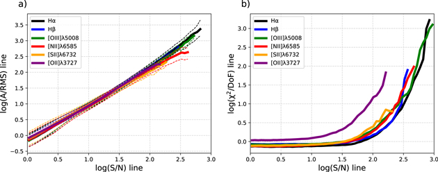
Figure 3. (a) Relation between S/Nline (Equation (1)) and  (Equation (2)) for a sample of spaxels taken from 300 random MaNGA galaxies in DR15. Different colors represent the median relation obtained for different strong emission lines, while the dashed curves represent the 16th and 84th percentiles. This panel demonstrates that the A/N closely tracks the S/N as measured by the DAP. (b) Relation between the χ2 per degree of freedom and S/Nline for the same sample of spaxels and set of strong emission lines as in panel (a). The χ2/DoF increases for high S/N as a consequence of template mismatch (i.e., a Gaussian is not a perfect model for a high-S/N emission line). We argue in the text that even in this regime the line fluxes measured by the MaNGA DAP are accurate.
Download figure:
Standard image High-resolution imageThe figure highlights the tight linear relation in log space between the two quantities across almost 3 dex in S/Nline for strong lines spanning a large fraction of the MaNGA wavelength range. This tight relation, which shows an increase in scatter only for S/Nline < 3, implies that the S/N computed by the DAP is equivalent to the more empirical A/N to very good accuracy. This scaling is indeed expected because most emission lines in MaNGA are unresolved, and their velocity dispersion is roughly comparable to one pixel in the spectral direction.
To check whether the fit residuals at the position of different emission lines are comparable with the error spectrum, we computed the χ2 per degree of freedom (dof) of the Gaussian fit in 15 pixel windows around the fitted position of each line center. In the right panel of Figure 3, we show the median relation between the  for each line and S/Nline. All strong lines considered follow a similar relation, except [O ii]λ3727, which suffers from worse χ2 at fixed S/Nline, possibly as a result of the difficulty in correctly fitting the unresolved doublet. For S/Nline < 30, the other strong lines show a roughly constant
  . At higher S/Nline, the
  increases sharply, up to three orders of magnitude. We interpret this as “template mismatch,” in the sense that our Gaussian model represents an increasingly worse representation of the observed line profiles at high S/N. In this regime, the χ2 could be lowered by fitting each emission line with more than one Gaussian component (e.g., Gallagher et al. 2019), but this goes beyond the scope of the current MaNGA DAP. We note a similar behavior in the
  over the full spectrum in both full-spectrum-fitting modules of the DAP, as shown in Figure 19 of Westfall et al. (2019); however, the discrepancies between model and data are orders of magnitude stronger in these small windows near each line.
We note that this increase in  does not mean that the fluxes obtained via Gaussian fitting are unreliable. In fact, we have checked that the fluxes obtained for Gaussian fitting agree exceedingly well with line fluxes obtained by simply summing the flux around the position of the line (SFLUX extension of the DAP MAPS files), as can be seen in Figure 4. For S/N < 3, we start to see a discrepancy between the two flux measurements, with Gaussian fluxes being higher on average. This effect is partially due to the fact that we fit a Gaussian with positive amplitude, while we allow negative summed fluxes. Exclusion of the negative summed fluxes from the comparison improves the median agreements at low S/N (not shown).
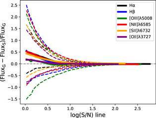
Figure 4. Relative difference between the flux derived from Gaussian fitting (FluxG) and that derived from zeroth-moment analysis (also referred to as summed flux, FluxS) as a function of line S/N (estimated from the Gaussian flux). In the case of [O ii]λλ 3737,29, both Gaussian and summed fluxes refer to both components of the doublet. The comparison demonstrates excellent agreement between Gaussian and summed fluxes for all lines in the high-S/N regime. At low S/N, Gaussian fluxes then tend to be higher than summed fluxes because we constrain Gaussian models to have positive amplitude.
Download figure:
Standard image High-resolution imageIn light of this discussion, we conclude that emission lines are statistically well fit by a single Gaussian model at low S/N. The increasing  does not imply that line fluxes from Gaussian fitting are unreliable in this regime, as can be demonstrated by a comparison with the nonparametric summed fluxes. Since S/Nline correlates very well with the empirically derived A/N, we suggest that, despite its simplicity, S/Nline is an excellent metric for the uncertainty in the fit. Henceforth, in this paper, S/Nline is used instead of A/N.
The typical line S/N of MaNGA data. To conclude this section, we present in Figure 5 the S/N distribution of the same sample of spaxels used in Figure 3, which is representative of the line S/N distribution in the MaNGA data. Only spaxels with S/N > 0 are plotted; that is, we do not plot the large number of spaxels that have no detected line emission according to our fitting procedure. Colored lines show the S/N distribution in three different radial bins. The radial variation of these S/N distributions highlights the decrease in S/N even in the strong nebular lines for  . We note that the MaNGA sample includes both star-forming and passive galaxies that are characterized by low-S/N line emission. In particular, the bimodality between star-forming and low-ionization emission-line regions (LIERs; Belfiore et al. 2016) is evident as a bimodality in the S/N of the Balmer lines, especially at small galactocentric radii.
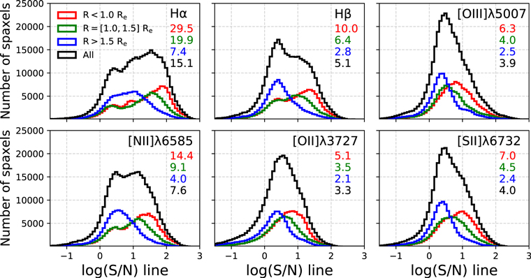
Figure 5. Distributions of emission-line signal-to-noise ratios for a large sample of spaxels (drawn from a random sample of 300 MaNGA galaxies in DR15). The black histogram includes all spaxels, while other histograms represent spaxels at different galactocentric distances ( , red; [1.0–1.5]
  , green;
  , blue). In color, on the right-hand side of each plot, we list the average S/N for each line in the associated radial range.
Download figure:
Standard image High-resolution image3.2. Idealized Recovery Simulations
In order to test the the presence of possible systematic errors in the recovery of emission-line parameters and the statistical correctness of the errors produced by the DAP, we have carried out a set of idealized recovery simulations. Four test galaxies were selected to span a wide range of stellar-continuum and emission-line properties (two star-forming blue galaxies and two red LIER galaxies). Considering all four galaxies, our mock data set consists of ∼5000 spaxels with S/N > 1 in Hα.
The MaNGA datacube for each galaxy was fit using the DR15 version of the DAP, and the best-fit model cube, including both continuum and emission lines, was used as a template for generating “mock” datacubes. For each spaxel in the model cube, Gaussian noise was added to the model spectrum, with a standard deviation given by the error vector in the input MaNGA data. Assuming the MaNGA DRP errors are accurate, this procedure generates mock cubes with the same noise level as the original data. Mock cubes with twice and half the noise level of the original data were also created.
All of the mock cubes were run through the MaNGA DAP in the same way as real MaNGA data. In particular, the same MILES-HC stellar templates were used to generate and then fit the mock cubes. In Section 4.4 we repeat this exercise using a different template set to fit the simulated data, and we discuss the effect of template mismatch.
In the ideal case, the fits to the mock datacubes would recover the input values of flux, velocity, and velocity dispersion for all emission lines with no bias, and the (1σ) errors for these quantities reported by the DAP should be equal to the standard deviation of the residuals between the output and input values. In other words, we expect  and
and  , where angle brackets denote averaging, std is the standard deviation,
  and qout are input and output values for a physical quantity, and errout is the DAP-provided error in qout. In this section, we will refer to
  as the normalized residual for quantity q.
In Figure 6(a) we plot the offset between input and output fluxes (in dex) as a function of measured (output) S/N for six strong emission lines ([O ii]λ3727, Hβ, [O iii]λ5007, Hα, [N ii]λ6584, and [S ii]λ6731). The plot demonstrates the existence of a small positive bias in the recovered flux for S/N < 6, which then becomes a sizable decrease in the recovered flux for the lowest S/N levels (∼2–3). Overall, the ability of the code to recover the input fluxes is better than 0.05 dex (12%) for S/N > 6.
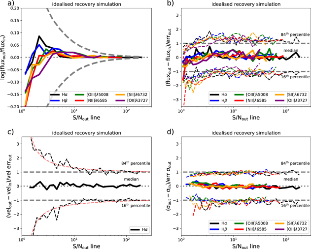
Figure 6. (a) Median offset (in dex) between the input and output fluxes of a parameter-recovery simulation. Different strong emission lines are represented by different colors, as noted in the legend. The dashed gray lines correspond to the level of offset consistent with random errors. (b) Median flux difference between the input and output flux, normalized by error in the output flux ( ), as a function of output signal-to-noise ratio (S/N = Flux/Error) of each line for an idealized simulation. The 16th and 84th percentiles of the distribution as a function of S/N are shown as dashed lines. In the case of perfect recovery, the median values should be zero and the 16th and 84th percentiles should be ±1. (c) Same as panel (b) but showing the velocity-normalized residuals versus the S/N for the Hα line. Only Hα is shown because the velocities of all lines are tied. The red lines represent fits to the 16th and 84th percentiles of the distribution given by Equation (3), which could be used to correct the errors. (d) Same as panel (b) but for the velocity dispersion. Overall, the results of these idealized simulations demonstrate that we are capable of recovering accurate fluxes down to low S/N and that the errors given by the MaNGA DAP are realistic for flux and velocity dispersion. In Equation (3) we provide a correction formula to obtain the correct velocity errors at low S/N.
Download figure:
Standard image High-resolution imageIn Figures 6(b)–(d), we plot the normalized residuals for the flux, velocity, and velocity dispersion as a function of the output S/N. The solid colored lines correspond to the median values of the normalized residuals in logarithmic bins of S/N, while the dashed lines represent the 16th and 84th percentiles. In all panels, in the case of perfect recovery, the median lines would lie at zero, and, assuming Gaussian errors, the 16th and 84th percentiles would follow horizontal lines at ±1.
From Figure 6(b), we observe that fluxes of all of the emission lines considered are recovered with negligible bias down to S/N ∼ 1.5. More notably, the errors are also correctly estimated, because the 16th and 84th percentiles closely follow the ±1 lines in normalized residuals. For S/N < 1.5, the flux is systematically underestimated. At these low S/N, the distribution of normalized residuals also deviates from a Gaussian, showing a long tail at low normalized residuals. We note that, while different lines cover different ranges in S/N, the behaviors of different lines are remarkably similar.
In Figure 6(c) we show the normalized residuals for the emission-line velocities as a function of Hα S/N. Only the Hα line is plotted in this panel, because all of the emission lines are fit with the same velocity. The figure shows that the input emission-line velocities are recovered with no bias down to S/N ∼ 1.5. However, the formal errors calculated by the DAP are underestimated for S/N < 10. In particular, at S/N ∼ 2, the output error is a factor of ∼3 lower than expected. At high S/N, on the other hand, the output errors are consistent with the scatter in the normalized residuals. The source of this underestimation likely lies in the fact that the formal error provided by pPXF for the gas fluxes is computed, for computational efficiency, from the covariance matrix of the gas emission templates alone. This implies that the uncertainties currently ignore the covariance between the fluxes (which are linear parameters in the fit) and the gas kinematics (which are nonlinear parameters). Proper uncertainties could be computed via bootstrapping at the expense of a significantly larger computation time, or by recomputing the covariance matrix with respect to all variables at the best-fitting solution.
In order to quantify this deviation, we have fit the observed relation with a simple functional form:

The resulting fit provides a very good representation of the data and is shown in light red in Figure 6(b). This correction is not applied to DR15 DAP output and needs to be taken into account by the user. We anticipate that users interested in fitting detailed kinematic models to the emission-line velocity field may need to take this correction factor into account.
Figure 6(d) shows the normalized residuals for the velocity dispersions of the different emission lines considered. The velocity-dispersion trends are similar to those observed for the flux and are indeed their likely cause, because the flux is positively correlated with dispersion. We observe remarkably good agreement in both the median and 16th and 84th percentile values down to S/N ∼ 1.5. Below that value, the dispersion shows a larger tail of negative normalized residuals.
Overall, idealized recovery simulations with no template mismatch demonstrate that the values and errors of flux and velocity dispersion can be recovered accurately with negligible bias down to S/N ∼ 1.5. The velocities can also be recovered reliably down to low S/N, but their associated errors appear to be underestimated for S/N < 10.
3.3. Error Statistics from Repeat Observations
In this section, we further analyze the error statistics for the emission-line measurements provided by the DAP by using repeat observations. In DR15, 56 galaxies have been observed more than once, mainly for the purpose of testing random and systematic errors (Westfall et al. 2019, Table 1).21 After processing these galaxies through the DAP, their MAPS files were transposed into the same world coordinate system, in order to account for small shifts in the integral-field unit (IFU) bundle positions and orientations between observations. The world coordinate system is derived by the MaNGA DRP by matching the MaNGA cubes to preexisting SDSS photometry in the advanced astrometry module (Law et al. 2016, Section 8), and it therefore takes into account small shifts and rotations of the IFU fiber bundles. In comparing repeat observations, we do not, however, take into account possible changes in the seeing conditions.
Similar to the procedure adopted to analyze the recovery simulations in the previous section, we calculate the normalized residuals as a function of S/N. Because for repeat observations we do not know the true value of any physical quantity, we define the normalized residual as  , where 1 and 2 refer to a pair of repeat galaxies, and err is the error in quantity q. Considering all repeat galaxies, we obtain a sample of ∼5 × 10⁴ pairs of spaxels with two independent measurements with S/N > 1 for Hα.
In Figure 7(a) we show the normalized flux residual as a function of S/N of the first galaxy in the pair. Following the same graphical conventions as in Figure 6, the solid colored lines represent the median, while the dashed colored lines represent the 16th and 84th percentiles as a function of S/N. The median residual is found to be close to zero. The 16th and 84th percentiles, on the other hand, are found to be close to ±1 at S/N ∼ 2 and show a systematic deviation toward larger values at higher S/N. This deviation is particularly evident for S/N > 10.
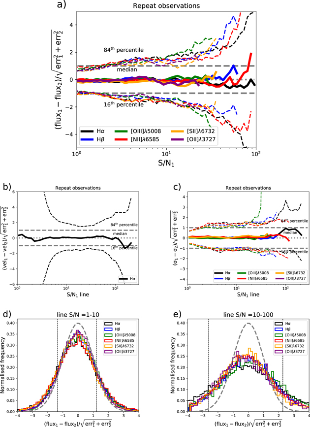
Figure 7. (a) Median flux difference between pairs of repeat observations normalized by rms error, that is,  as a function of signal-to-noise ratio (S/N = Flux/Error) of each line. Different strong emission lines are represented by different colors, as noted in the legend. The 16th and 84th percentiles of the distribution as a function of S/N are shown as dashed lines. If the output errors are correct, the 16th and 84th percentiles of the normalized residual distribution should be ±1. (b) Same as panel (a) but showing the velocity-normalized residuals versus the S/N for the Hα line. Only Hα is shown because the velocities of all lines are tied. (c) Same as panel (a) but for the velocity dispersion. (d) Distribution of normalized flux residuals in the S/N range [1–10] for six strong emission lines, listed in the legend. The gray dashed line represents the expected distribution assuming Gaussian errors. The black vertical dashed lines are the 16th and 84th percentiles of the Hα normalized residual distribution. If the errors are correct, these values should lie at ±1. (e) Same as (b), but for the S/N range [10–100]. Note that in this regime the normalized residual distributions are broader and the errors appear to be underestimated.
Download figure:
Standard image High-resolution imageIn Figures 7(b) and (c), we show the normalized residuals as a function of S/N for the velocity and velocity dispersion. For velocity, the errors are underestimated at all S/N, with the worst discrepancy at low S/N, similar to what was found in our study of idealized simulations in the previous section. Different from what was seen in the previous section, the errors also diverge from expectations at high S/N (S/N > 20–30), while they appear to be underestimated by a factor less than 2 in the range S/N = [6, 50]. The velocity dispersion appears to be much better behaved, with no evidence for large error underestimation until S/N > 100. Interestingly, for S/N = [1, 2], the errors appear to be overestimated.
Figure 7(d) shows the distribution of normalized residuals for six strong lines (see legend) in the S/N range [1–10]. The gray dashed line shows a normalized Gaussian of unit standard deviation, which represents the theoretical expectation in case of ideal error measurements. In Figure 7(d) we show as vertical black dashed lines the 16th and 84th percentiles of the observed distribution for Hα (1.22 and −1.35, respectively). We note that, although the data presents slightly non-Gaussian tails, it is well fit to first order by a Gaussian with standard deviation 1.25 (fit not shown).
Figure 7(e) is the same as Figure 7(d), but represents the S/N range [10–100]. As already evident in Figure 7(a), at this S/N level, either the errors are underestimated by a factor of 2–3, or some other systematic enters into the comparison of repeat observations.
Because this large error underestimation is not seen in the idealized recovery simulation, we consider possible systematic effects that could cause this. First, as already seen in Section 3.1, at S/N > 20–30, our Gaussian model may be insufficient to accurately fit the line profiles in real data, leading to higher normalized residuals and, possibly, underestimated errors. Second, regions of bright line emission tend to be clumpy, and the measured fluxes are therefore particularly sensitive to differences in point-spread function (PSF). In this case, the increased error in flux is due to intrinsic scatter in the amplitude, and not to larger errors in the recovered velocity dispersion, which would be in agreement with the findings from Figure 7(c). The same effect would be caused by small astrometric misalignments between repeat observations.
We gained some insight into these issues by visually inspecting difference and normalized residuals maps for different pairs of repeat observations. This exercise clearly revealed that the largest normalized residuals are indeed associated with bright and clumpy line emission. We have therefore performed a simple test to quantify the effect of astrometric offsets and PSF differences. One of the galaxies showing the largest differences in normalized residuals was selected as an example. For this galaxy, we considered the output of the MaNGA astrometry module, which matches the MaNGA IFU data to the underlying SDSS photometry in order to correct for small deviations of the rotation and centroid position of the MaNGA IFU ferrules in a given exposure due to the mechanical tolerance of the ferrule and rotational clocking pin holes. We artificially added random error to the best-fit astrometric solution, consistent with the uncertainty calculated by the astrometry module (typically about 025 and 0
1 for the rotational and translational components, respectively). A datacube was then produced, following the usual MaNGA reduction recipes, and fit using the DAP. We compared the output produced by this datacube with additional astrometric error to the reference datacube generated for DR15. At low S/N, the dispersion in line fluxes between the two datacubes is negligible, but it flares at high S/N in a fashion consistent with that observed in Figure 7(a). In particular, we find that astrometric errors consistent with those expected by registering MaNGA data to SDSS photometry are sufficient to explain the observed increase in the error budget in repeat observations.
3.4. Summary and Recommendations with Regards to Errors
In summary, recovery simulations demonstrate that the errors for flux and velocity dispersion of different emission lines behave in a statistically correct fashion down to S/N ∼ 1.5. Errors in the velocity are underestimated for S/N < 10, and the source of this discrepancy is not know at the time of writing. Equation (3) quantifies this underestimation and can be utilized to rescale the errors based on the outcome of the recovery simulation. In DR15 we leave it to the user to apply this correction if deemed necessary to their science goal.
These trends are largely confirmed by the analysis of repeat observations. Repeat observations, however, also show underestimation of the errors in the high-S/N regime. We have demonstrated that this trend can be entirely explained by small astrometric errors in individual exposures, which are consistent with the uncertainties derived by the MaNGA DRP astrometric registration routine. In light of this discussion, we leave it up to the user to consider whether adding this extra error contribution is advisable for their specific science goal.
4. Systematic Errors from the Modeling of the Continuum
In the section, we address the systematics on emission-line properties that arise from the modeling of the continuum. We present MILES-HC, the stellar library used to fit the MaNGA data in DR15, and discuss the differences in the recovered emission-line properties obtained using several different SSPs.
4.1. Stellar and SSP Template Libraries
In the following section, we briefly outline the characteristics of the spectral libraries that we will discuss and compare in this paper.
Hierarchically clustered MILES templates (MILES-HC). As discussed in Section 5 of Westfall et al. (2019), we have applied a hierarchical clustering algorithm to the MILES stellar library, which consists of 985 stars covering the wavelength range 3525–7500 Å (Sanchez-Blazquez et al. 2006; Falcón-Barroso et al. 2011). The clustering algorithm subdivides the stars in the MILES library into a number of groups that are defined to be maximally different from each other. Forty-nine such groups are generated, and a composite spectrum is obtained for each group as the average of the spectra of the contributing stars. These 49 spectra were visually inspected, and seven of them were removed because of artifacts or the presence of emission lines (in flaring late-type stars), leading to a total of 42 stellar templates. The resolution of the MILES library has been independently derived by Beifiori et al. (2011) and Falcón-Barroso et al. (2011) and is 2.54 Å (FWHM). This library is used in generating all of the DAP DR15 data products.
Maraston 2011 SSP models based on MILES (M11-MILES). These SSP are generated using the MILES stellar library by the Maraston stellar-population synthesis code (Maraston & Strömbäck 2011).22 A total of 110 models are used with ages ranging from 6.5 Myr to 15 Gyr, three metallicities (Z = 0.01, 0.02, 0.04), and a Salpeter IMF. The spectral resolution is the same as that of the MILES library (2.54 Å FWHM).
Vazdekis MIUSCAT SSP Models (MIUSCAT). This is a set of 72 SSP models generated according to Vazdekis & Ricciardelli (2012)23 with a Salpeter IMF (unimodal IMF with slope = 1.3) and a set of 24 ages (0.0631, 0.0794, 0.1000, 0.1259, 0.1585, 0.1995, 0.2512, 0.3162, 0.3981, 0.5012, 0.6310, 0.7943, 1.0000, 1.2589, 1.5849, 1.9953, 2.5119, 3.1623, 3.9811, 5.0119, 6.3096, 7.9433, 10.0000, 12.5893 Gyr) and three metallicities ([M/H] = −0.4, 0.0, 0.22). MIUSCAT extends the wavelength range of MILES to cover the full range 3465–9469 Å by making use of the near-infrared CaT library of Cenarro et al. (2001). Stellar spectra from the Indo-US stellar library are used to fill in the gap left between the MILES and CaT spectral ranges and also to extend toward the blue and red the wavelength coverage of the MILES and CaT libraries, respectively. The spectral resolution is the same as the MILES library, as the higher-resolution CaT and Indo-US libraries are convolved to the MILES spectral resolution. The MaNGA VAC generated by the Pipe3D team also uses a subset of MIUSCAT templates for spectral fitting, although the exact set of templates differs from the ones described above.
Bruzual and Charlot SSP models based on STELIB (BC03). This is the set of 40 Bruzual & Charlot (2003) models used in the MPA-JHU catalog for the SDSSDR4.24 The SSP templates cover a range of 10 ages (0.005, 0.025, 0.101, 0.286, 0.640, 0.904, 1.434, 2.500, 5.000, 10.000 Gyr) and four metallicities (Z = 0.008, 0.004, 0.02, 0.05) using a Chabrier IMF. The SSP models are based on the STELIB stellar library (Le Borgne et al. 2003) and have nominal spectral resolution of 2.3 Å. These SSP models are different from the BC03 SSP based on MILES used to produce the MPA-JHU value-added catalog for later data releases, such as the latest DR8 version.25
4.2. Choosing between Stars and SSPs
In this section, we investigate the consistency between the MILES-HC stellar library used in DR15 and the SSP models described in the subsection above. SSP models prescribe parameterized combinations or interpolations between elements of stellar libraries based on physical models of stellar interiors, atmospheres, and their evolution (isochrones). To the extent that these physical models are incomplete or simply inaccurate, one may worry about whether SSP and stellar spectra are consistent in both overall shape and in the details of their absorption features. SSP models based on observed stellar libraries mitigate, for example, incomplete line lists in synthetic spectra, but suffer problems of library incompleteness and stellar misclassification. Library incompleteness is a general concern for all continuum-fitting methods, and it is the specific concern motivating the work in this section.
In particular, the lack of hot (O-type) stars in the MILES library potentially undermines our ability to fit young stellar populations with MILES-HC. The hierarchical clustering performed on the spectra may further dilute the blue continua of the few B stars present in MILES. While O-star spectra are largely featureless, their very blue continua cannot be reproduced by a linear sum of other stellar spectra. A common solution to this problem, within the pPXF framework, is to allow the inclusion of additive or multiplicative polynomials in the fit. These polynomials are generally of low order to avoid any effect of the polynomial on the spectral features of individual absorption lines.
However, hot stars do have some critical features, notably in their hydrogen and helium lines, that have distinct and systematic changes with temperature. These changes in stellar absorption lines include the EW, the core width (due to rotation and winds), and the relative strength and shape of the wings (due to the Stark effect). None of these are modified by multiplicative polynomials, and only the EW (not the shape) can be modulated by additive polynomials. Further, because of the different and nonlinear temperature dependence of these features, it is not possible to accurately simulate spectra containing O stars with a library that does not include these stars. For a library with such a deficiency, we would expect to see Balmer lines that are too narrow and a deficiency of He absorption. Because this will lead to systematics in the continuum model at the location of key emission lines, the amplitude of such systematics is important to assess.
We therefore test the ability of the MILES-HC library to reproduce different stellar populations by fitting the BC03 SSP models of different ages (and solar metallicity) with MILES-HC spectra. The fit has been performed in three ways: (1) with no polynomials, (2) with an eighth-order additive polynomial, and (3) with an eighth-order multiplicative polynomial. Aside from the polynomial type, we perform this fit in the same way as the first (i.e., the stellar kinematics) fitting stage of the DAP. In each case, we compute the residual between the best-fit model and the input SSP and compute the resulting rms over the wavelength range 3700–7400 Å.
The fractional rms (i.e., the standard deviation of output–input/input) calculated over ∼40 Å windows is shown in Figure 8 for BC03 templates of different ages fitted with no polynomials.
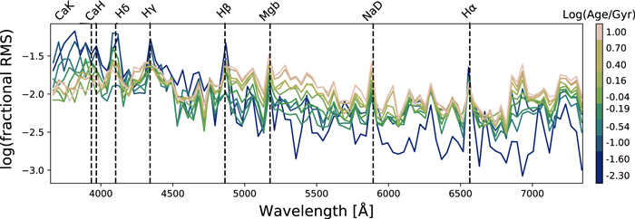
Figure 8. Fractional rms of the residuals obtained when fitting BC03 SSP models of different ages (and solar metallicity) with MILES-HC stellar templates (and no polynomials). The residuals are computed in 40 Å bins spanning 3650–7400 Å and the ages of the templates considered as given in the color bar. Prominent metal absorption lines (e.g., Mgb and NaD) lead to localized increases in the rms, especially for the older SSPs. An increase in rms is also evident at the positions of Balmer series lines, especially at young ages.
Download figure:
Standard image High-resolution imageThe figure demonstrates that the overall spectral shape of the BC03 SSPs are well fit by MILES-HC, with median residual rms values of 10−2.0. The largest rms values are seen both at the blue end of the spectrum at very young ages and in very localized wavelength regions, generally corresponding to notable absorption lines. Balmer series lines are particularly problematic and increasingly so at young ages. Metal lines (such as Mgb and NaD), on the other hand, are fit worse at older ages. The inclusion of polynomials does not lead to an overall improvement of the fit quality, although it does have an effect on the fit around the Balmer and helium lines.
Figure 9 compares the fits of the MILES-HC library to the BC03 SSPs for ages of 5 and 25 Myr with and without polynomials. This figure is worth careful scrutiny. Inspection reveals MILES-HC underpredicts the hydrogen line depths, increasingly for lower-order lines. This is mostly ameliorated by either additive or multiplicative polynomials, which do a good job of matching the wings but fail to match the core. The same relative statements are true for the 25 Myr SSP, but the amplitudes of the differences are decreased, that is, the MILES-HC fit is substantially better on its own without polynomials. In contrast, the MILES-HC fits overpredict He i and underpredict He ii lines for BC03 for both ages. Polynomials do little to help remedy the mismatch in EW and often degrade the quality of the fit.
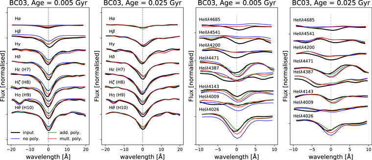
Figure 9. Zoom-in around the hydrogen Balmer (left) and helium (right) lines. The black spectrum corresponds to the input SSP (from BC03) being fit using the MILES-HC library, and the colored lines represent the best fits (blue, with no polynomials; green, with eighth-order additive polynomials; red, with eighth-order multiplicative polynomials). SSPs of two different ages (5 and 25 Myr) are shown.
Download figure:
Standard image High-resolution imageWe can interpret the overpredicting of the He i and the underpredicting of He ii lines as being due to the lack of very hot O stars in MILES-HC. B stars are the hottest stars in the library, and they do not have He ii lines. If MILES-HC lacks templates with strong He ii lines, then the fit will use more B stars to compensate for the spectral shape and end up overfitting He i, while still not producing the He ii features.
A detailed accounting of the stellar templates (and their weights) that go into the specific SSPs would be one way to make progress on this question, but this critical “deconstruction” of SSPs is beyond the scope of this paper.
We conclude that even with additive or multiplicative polynomials, MILES-HC is likely to have small systematic residuals in the cores of the hydrogen lines that lead to emission-line overestimates at the very youngest ages. The systematics for helium lines are more significant and varied, and in some cases are minimized without including polynomials. Polynomials do not significantly improve the overall match of the spectral between SSPs and stellar templates, which is excellent except for the youngest ages for λ < 4000 Å.
4.3. Effects of the Continuum Model on Line Fluxes
In order to explicitly test the effect on measured emission-line fluxes caused by the use of different stellar-continuum models, we fit a subset of DR15 MaNGA datacubes with the three sets of SSPs discussed in Section 4.1, in addition to the MILES-HC fit performed in DR15. In particular, we used SSPs to perform the second fitting stage in the DAP, but not for the extraction of the stellar kinematics, for which stars are generally recommended. When necessary, the difference between the intrinsic spectral resolution of the MILES stars and that of the SSP templates used for the second fitting stage has been taken into account.
The SSP fits were carried out for a sample of 15 galaxies, evenly sampling the NUV − r versus  plane, in order to have access to a wide variety of stellar populations. We only considered galaxies with line emission (including extended LIER galaxies on the red sequence). Considering the entire galaxy subsample, we obtain ∼2 × 10⁴ spaxels with Hα S/N >1.
In Figure 10 we compare the emission-line fluxes obtained using MILES-HC for both fitting stages (i.e., the DR15 data products) with the fluxes obtained after switching to an SSP template for the second fitting stage. The flux ratios are presented as a function of line S/N for different strong lines. The dashed gray lines represent the level at which the flux difference is comparable to the random error.
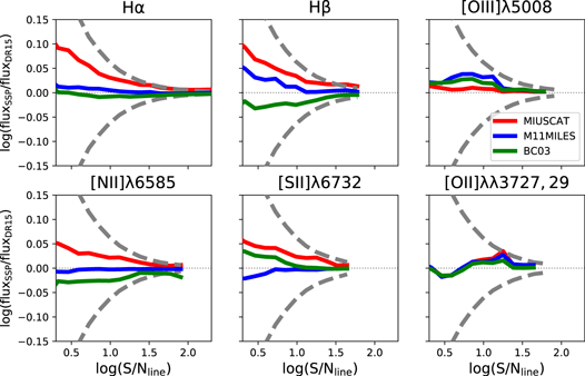
Figure 10. Ratio in the emission-line flux (in dex) obtained when modeling the continuum with various SSP templates (MIUSCAT, red; M11-MILES, blue; BC03, green) with respect to the fluxes obtained in DR15 (which uses MILES-HC templates) as a function of line S/N. The dashed gray lines correspond to the level where the flux discrepancy is equal to the random error. The largest systematic discrepancies are found for Balmer lines at low S/N. Low-S/N line emission in MaNGA is generally associated with low-EW line emission, so this figure looks equivalent to the flux discrepancy plotted as a function of EW instead of S/N.
Download figure:
Standard image High-resolution imageFigure 10 shows a number of interesting features. For the Balmer lines (Hα and Hβ are shown in the figure), different templates give systematically different line fluxes because of the different best-fit stellar Balmer absorptions, especially at low S/N. MIUSCAT prefers deeper Balmer absorption, leading to larger Balmer line fluxes than MILES-HC. BC03 and M11-MILES lead to better agreement with DR15 for Hα but show significant differences in Hβ. It is interesting to note that the systematic discrepancies are substantial (up to 0.1 dex at S/N = 2 between DR15 and MIUSCAT). They are, however, smaller than the random errors at low S/N, while they become comparable to (or larger than) the random error at high S/N. We have checked the behavior of the flux differences as a function of EW of the lines, and the resulting plot is very similar to Figure 10, especially for the Balmer lines, because S/N largely tracks the EW.
On the other hand, for metal lines, such as [O iii]λ5007, [S ii]λ6732, and [O ii]λλ 3727,29, the discrepancies between fluxes obtained with different templates are less extreme and do not correlate as well with line S/N. [N ii]λ6585 and [S ii]λ6732 stand out from the other metal lines for showing comparatively larger discrepancies. In Figure 11 we show some example fits to the spectral regions around Hα and the [N ii] doublet for the central spaxel of four galaxies (low-mass blue, 7815–6101; massive blue, 8138–12704; low-mass red, 8329–1901; high-mass red, 8258–6102) spanning a range of properties in the NUV − r versus  plane. These example fits highlight the previously discussed differences in the core of the Hα line, but also the resulting effect on the nearby [N ii] lines, which are the outer edges of the Balmer absorption wings. For example, the BC03 templates generate best-fit models that have substantially different line wings from those of other template sets, therefore affecting the [N ii] flux in addition to Hα.
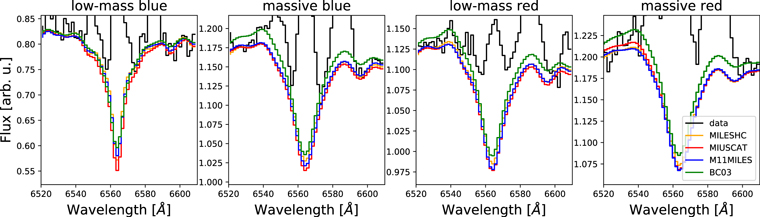
Figure 11. Continuum fits around the Hα and [N ii]λλ 6548,84 for the central spaxels of four example galaxies spanning different regions of the NUV − r versus  plane using different stellar (MILES-HC) and SSP (M11-MILES, MIUSCAT, BC03) templates. Note how MIUSCAT and M11-MILES prefer deeper Balmer absorption-line cores and how BC03 displays significantly different line wings, which affect the continuum under the [N ii]λλ 6548,84 doublet. The galaxies in the figure are low-mass blue, 7815–6101; massive blue, 8138–12704; low-mass red, 8329–1901; and massive red, 8258–6102.
Download figure:
Standard image High-resolution imageAlthough these flux discrepancies are smaller than the random error, they are systematic and behave differently for the different lines considered, therefore leading to biases in the derived line ratios. In Figure 12 we show the differences in dex for several line ratios and other derived quantities between the cases fit with SSPs and DR15 as a function of EW(Hα). In the first row, we show the Balmer decrement (Hα/Hβ) and two classical BPT (Baldwin–Phillips–Terlevich; Baldwin et al. 1981) line ratios ([N ii]/Hα and [O iii]/Hβ). At low S/N, the Balmer decrement measured with MIUSCAT and M11-MILES differs substantially from that inferred in DR15 or using BC03. Estimating E(B − V) using an intrinsic ratio  = 2.86 and a Calzetti (2001) extinction curve, we see that deviations up to 0.1 dex are evident at EW(Hα) ∼ 2 Å, growing worse at even lower EW. Regarding the BPT line ratios, [N ii]/Hα is relatively unaffected by template choice, possibly because the vicinity of the two lines means they are affected by the best-fit continuum shape in a correlated way. [O iii]/Hβ, on the other hand, displays significant differences for low-EW lines (there is a 0.2 dex difference between MIUSCAT and DR15 at EW(Hα) ∼ 2 Å). These biases will have a measurable effect on the BPT diagram positions of low-EW regions, which tend to be associated with LIER emission and diffuse ionized gas.
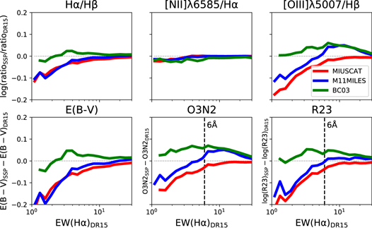
Figure 12. Difference in dex between specific line ratios when the spectral fitting is preformed with various SSP templates (MIUSCAT, red; M11-MILES, blue; BC03, green) with respect to the line ratios obtained in DR15 (which uses MILES-HC templates) as a function of line EW.  is computed from the Balmer decrement assuming an intrinsic ratio
  = 2.86 and a Calzetti (2001) extinction curve. In the case of E(B − V), the plotted difference is in magnitudes. The R23 index is computed after correcting for dust attenuation, while the other indices are not corrected.
Download figure:
Standard image High-resolution imageIn the bottom row of Figure 12, we also show two metallicity-sensitive indices often employed in the literature, O3N2 = ([O iii]λ5007/Hβ)/([N ii]λ6583/Hα) (Pettini & Pagel 2004) and R23 = ([O ii]λλ 3727,29 + [O iii]λλ 4959,5007)/Hβ (Pagel et al. 1979). While O3N2 is relatively insensitive to dust extinction, we correct the measured line fluxes for extinction when computing R23. It is evident from the figure that discrepancies larger than 1/10th of a dex are present at low EW for both indicators. A cut on EW(Hα) > 6 is sometimes performed in studies of ISM metallicity in order to minimize the contamination from gas not directly associated with H ii regions (Sánchez et al. 2014). Here we show this threshold as a dashed black line for these two indicators in Figure 12, demonstrating for larger EWs that the systematic effects from the choice of continuum templates are nonnegligible. This exercise demonstrates that care is needed when comparing results from IFU surveys calculating emission-line fluxes with different underlying stellar or SSP models.
In the Appendix we perform a similar comparison on the line fluxes measured by the DAP and the Pipe3D VAC for DR15. The DAP and Pipe3D differ in many fundamental aspects besides the choice of continuum templates, so it is more difficult to attribute discrepancies to just one factor. However, for some line ratios (like Hα/Hβ and [O iii]/Hβ), we find discrepancies between the results of the two pipelines that are comparable, at least qualitatively, with those between the DAP DR15 run and the DAP run utilizing MIUSCAT templates. These differences may therefore be attributed at least partly to the different choice of continuum templates in the two pipelines.
However, while the results in this section show no strong effect of template choices on the [N ii]/Hα, we do find significant discrepancies for this line ratio between the DAP and Pipe3D. This fact is discussed further in Appendix A.2.
4.4. Simulating the Effect of Template Mismatch
The aim of this section is not to select the “correct” set of templates, but simply to quantify the effect of different templates on the resulting emission-line fluxes. In general, we cannot determine which set of templates is the correct one for our galaxy data, so we devise an artificial exercise similar to the recovery simulation presented in Section 3.2 to study the effect of using the “wrong templates” in the presence of noise.
In particular, we take the best-fit model from the previous section based on a set of SSP templates and add noise in the same way as was done in Section 3.2. Here we discuss the results of using mock datacubes generated using the MIUSCAT best-fit models, which are then fit using the standard DR15 approach (i.e., using the MILES-HC library). In light of the results of the previous section, we expect the recovered Balmer line fluxes to be lower than the input ones on average, given the preference for MIUSCAT to fit deeper Balmer absorption features.
Figure 13 demonstrates this effect. The recovered Hα and Hβ fluxes are indeed systematically lower than the input ones. It is interesting to note, however, that while the median flux is systematically biased, the 16th and 84th percentiles still approximately correspond to ±1 with respect to the median, indicating that template mismatch does not dramatically affect the statistical validity of the emission-line flux errors. At low S/N, we also observe a bias in the recovered fluxes, in the sense that the flux tends to be underestimated, as already noted in Section 3.2 (see Figure 6(a)).
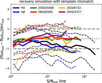
Figure 13. Difference between the input and output fluxes, normalized to the error, for a parameter-recovery simulation that includes template mismatch (see text). The setup of the figure is the same as Figure 6(a). The solid colored lines represent the median, and the dashed colored lines the 16th and 84th percentiles of the normalized residual distributions for the different strong lines considered. The Balmer lines (Hα in black and Hβ in blue) display the expected systematic offset at high S/N.
Download figure:
Standard image High-resolution image5. Systematics from Algorithmic Choices
In this section we address the systematic errors on emission-line parameters that may result from specific algorithmic choices. In particular, we study the effect and importance of the polynomial corrections adopted in DR15 and critically assess the strategy of simultaneously fitting the continuum and emission lines in the second fitting stage of the DAP. We also explore different schemes for tying the velocity and velocity dispersion of different emission lines and compare them to the approach we have followed in DR15.
5.1. Multiplicative Polynomials
In this section, we assess the role and importance of multiplicative polynomials in the second fitting stage of the DAP (the simultaneous fitting of continuum and emission lines). A complementary discussion of the role of additive polynomials during the first fitting stage of the DAP (stellar kinematics) is presented in Section 7.3.3 of Westfall et al. (2019). We remind the reader that the multiplicative polynomials are only applied to the stellar-continuum templates and not to the emission-line (Gaussian) templates. In this sense, their effect on the line fluxes is only indirect. We nonetheless address this issue here as a check on the quality of our continuum model and for its relation to the overall flux calibration of the MaNGA survey.
5.1.1. Role of Polynomials
The inclusion of polynomials during the pPXF fit may be advantageous for several reasons:
- 1.Multiplicative polynomials can compensate for residual differences in the relative flux calibration of the science data with respect to the stellar templates. Assuming the spectral templates are perfectly calibrated (and in the presence of negligible extinction), one may use the shape of the recovered polynomials to test the quality of the flux calibration of the data.
- 2.Polynomials can mimic the shape of canonical extinction curves.
- 3.Polynomials can provide low-order corrections to the stellar-population models, which may be especially valuable when theoretical stellar spectra are used. In addition, they can help to reproduce the shape of the spectra of stars that are not present or are underrepresented in the library used (as we have discussed in Section 4.2).
5.1.2. Typical Shape of the Polynomial Correction in DR15
In this section, therefore, we start by looking at the typical shapes of the multiplicative polynomials used in the second fitting stage for the DR15 DAP run. To do so, we selected a random sample of 100 DR15 galaxies and reconstructed the multiplicative polynomials used in each of their spaxels. In Figure 14 we show the shape of the median multiplicative correction applied as a function of rest-frame wavelength. The sample of galaxies is subdivided into two mass bins (red for  blue for
  ) and the shaded areas correspond to the 16th and 84th percentiles of the distribution. We also show in black the expected multiplicative correction for a Calzetti extinction curve and two values of E(B − V).26
The extinction curves are scaled arbitrarily to the median of the polynomial corrections to highlight the similarity in relative shape.
) and the shaded areas correspond to the 16th and 84th percentiles of the distribution. We also show in black the expected multiplicative correction for a Calzetti extinction curve and two values of E(B − V).26
The extinction curves are scaled arbitrarily to the median of the polynomial corrections to highlight the similarity in relative shape.
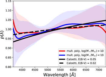
Figure 14. Median multiplicative polynomial correction applied to the best-fit continuum templates calculated for all spaxels in a sample of 100 random galaxies from DR15. Red and blue solid lines correspond to the median correction for  and
and  galaxies, respectively. The shaded regions correspond to the 16th and 84th percentiles. The black curves represent a Calzetti (2001) extinction curve with different values of E(B − V).
Download figure:
Standard image High-resolution imageThe trends observed in the figure can be qualitatively interpreted as follows. The massive bin contains a larger number of passive galaxies, which are largely devoid of gas and thus suffer lower extinction. The shapes of the polynomials are consistent with the values of E(B − V) measured for the continuum by full spectral fitting in the outskirts of MaNGA galaxies (Goddard et al. 2017).
5.1.3. Deviations from Smooth Polynomial Shapes and Consequences for Flux Calibration
The key features in Figure 14 are the deviations from the expected smooth extinction curves, namely the upturn in the mean correction at the blue end of the MaNGA wavelength range and a similar downturn redder than 7000 Å. We determined that these deviations are not due to imperfections in the MaNGA flux calibration for the following reasons.
First, the upturn in the blue occurs at different observed wavelengths for galaxies at different redshifts. For example, if one considers massive galaxies in the MaNGA primary and secondary samples, which are selected in the same fashion but separated by a small redshift interval, the blue upturn moves to longer observed wavelength in the secondary sample. If the upturn was due to imperfections in the MaNGA flux calibration derived from standard-star spectra, it would always appear at the same observed wavelength. Second, the downturn observed redder than 7000 Å occurs in the middle of the MaNGA spectral coverage (but at the edge of the spectral coverage of MILES-HC) and is therefore more likely to be originating from the MILES-HC than the MaNGA data.
In order to test whether imperfect relative flux calibration of the MILES-HC library is responsible for the deviations observed in Figure 14, we selected one test galaxy (a massive red galaxy, 8258–6102, with good S/N throughout) and examined the stacked polynomial shapes obtained after fitting the galaxy with different template sets. The results are presented in Figure 15. It is interesting to note that between 4000 and 7000 Å, MILES-HC (labeled DR15), M11-MILES, MIUSCAT (all based on MILES stars), and BC03 (based on STELIB) agree to better than 10%. Bluer than 4000 Å, BC03 presents a downturn, while both M11-MILES and MILES-HC show an upturn. MIUSCAT, on the other hand, gives rise to a flattening. It should also be noted that the downturn at 7000 Å is present both in MILES-HC and M11-MILES, pointing toward a problem with the MILES stars.
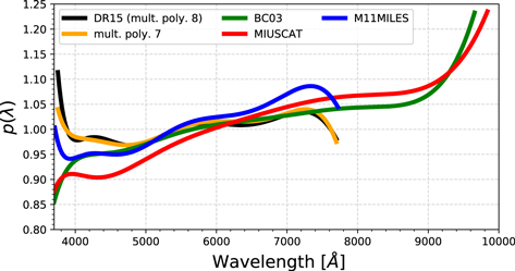
Figure 15. Median multiplicative polynomial correction for one massive elliptical test galaxy (8258–6102), fit using different stellar and SSP templates. An upturn in the polynomial correction is evident for  for the DR15 (MILES-HC, in black) and the M11 MILES (in blue) templates. We attribute this upturn to an issue in the flux calibration of the MILES stellar library. Interestingly, the same effect is not as evident for the MIUSCAT (in red) templates, which are also based on MILES stars. The shape of the downturn is independent of the polynomial order used (in orange we show the result of using seventh-order multiplicative polynomials and MILES-HC). In the far red (λ > 9000 Å), we note a red upturn, picked up both by BC03 (in green) and MIUSCAT. For the moment, we cannot exclude that this red upturn is an artifact of the MaNGA flux calibration.
Download figure:
Standard image High-resolution imageTo check the behavior of the code at the edges of the wavelength range, we changed the degree of multiplicative polynomials from eight to seven (i.e., from even to odd parity). If the behavior of the polynomials at the edges was entirely dictated by the fit within the central wavelength region, we would expect that a change of parity would lead to a change in symmetry of the recovered multiplicative correction, which is however not seen in Figure 14. We concluded, therefore, that the offsets seen at the edges of the fitted MaNGA wavelength range are likely to be real.
It is possible that MILES-HC suffers from the lack of hot stars, including blue horizontal branch stars. These stellar types may have been accounted for differently by different SSP models, generating the discrepancy observed between BC03, MIUSCAT, and M11-MILES at the blue edge of the optical wavelength range.
Interestingly, the SSP templates that extend redder than 9000 Å show the need for an upward correction to match the MaNGA data. The presence of this red upturn has been identified via visual inspection in some of the MaNGA spectra. Since this spectral range is not fit in DR15, we postpone further study of this potential systematic effect.
5.2. Combined Effect of Masking and Polynomials
The MaNGA DAP implements simultaneous fitting of emission-line and continuum templates following the recommendation from previous work (Sarzi et al. 2005; Oh et al. 2011). Sarzi et al. (2005), in particular, demonstrated the advantage of this algorithmic choice when dealing with the limited wavelength range of the SAURON data, where the emission lines lie in close vicinity to the key metallicity- and age-sensitive features. In Section 4.3, however, we have demonstrated that, even by performing simultaneous fitting, residual degeneracies between Balmer absorption and line emission are still present, leading to noticeably different best-fit models when using different template libraries. In this section, therefore, we perform some illustrative tests to evaluate the impact of the masking on the recovered best-fit continuum under the Balmer lines.
We first examine the difference between the best-fit continua obtained by the first and second fitting stages in the DAP for the central spaxels in four test galaxies (Figure 16, same galaxies as in Figure 11). A difference between the two best-fit stellar-continuum models in this comparison may be due to either the effect of masking (emission-line regions are masked in the first fit but not in the second) or the difference in the use of polynomials (additive polynomials in the first fit and multiplicative polynomials in the second fit). In Figure 16 we plot the difference between the two best-fit models normalized by the input spectrum. At the wavelength of a specific emission line, this can be interpreted as the fractional error in the amplitude of the line introduced by these different choices in continuum fitting.
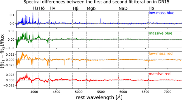
Figure 16. Spectral differences between the best-fit stellar continuum in the first fitting stage of the DAP and that of the second fitting stage normalized by the input spectrum. At the position of specific emission lines, the y-axis value can be interpreted as the fractional error in the amplitude of the line due to the different continuum models. The four spectra shown are taken from the central regions of different test galaxies, spanning a range in stellar mass and color (low-mass blue, 7815–6101; massive blue, 8138–12704; low-mass red, 8329–1901; massive red, 8258–6102). The first fitting stage masks regions potentially contaminated by emission lines and allows the use of additive polynomials, while the second fitting stage performs simultaneous fitting of gas and stellar templates and makes use of multiplicative polynomials. The main differences between the best fits from the two stages are seen in regions of strong Balmer and metal absorption.
Download figure:
Standard image High-resolution imageThe largest deviations are seen in regions corresponding to strong absorption lines (like the NaD doublet, evident in all four examples except the low-mass blue galaxy) and the Balmer absorption lines. However, in the case of Balmer lines, the differences can be both positive and negative. We attribute this behavior to the different implementation of polynomials in the two fitting stages. In the case of the low-mass blue galaxy, where the most prominent absorption features are the Balmer lines, additive polynomials lead to shallower absorption-line profiles, which result in positive residuals at the positions of the Balmer lines in Figure 16. For the higher-mass galaxies, other metal absorption lines dominate the spectrum and therefore determine the shape of the additive polynomials, causing positive, null, or negative residuals around the Balmer lines. We note that the deviations observed in the low-mass blue galaxy are much larger than those observed in the red galaxies, with significant changes already seen at Hβ (∼3%) and increasing to 13% at H.
A cleaner test to isolate the effect of masking is to apply the same type of polynomials to both the first and second fitting stages. We have therefore repeated the exercise just described by using eighth-order multiplicative polynomials for both fitting stages. The resulting normalized flux differences are shown in Figure 17 and look substantially different from Figure 16. Now the differences around metal absorption lines are reduced, and the Balmer lines correspond to the largest residuals (of the order of ∼1%–2%). These are again stronger for the high-order Balmer lines (in particular Hδ and Hγ). Integrating over the line profile, we see the systematic differences in Hα flux are less than 2%, which is negligible in most cases when compared to the discrepancies caused by changes in the template library. However, the changes in measured fluxes are more substantial for the high-order lines.
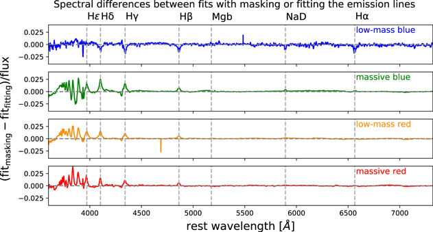
Figure 17. Same as Figure 16, but using eighth-order multiplicative polynomials in both fitting stages of the DAP. The difference between the two best-fit models is only driven by the masking of the emission lines in the first stage (in the second stage, emission lines are fit at the same time as the continuum). Small differences (<2% of the Hα flux) can be seen in the best-fit models at the position of the Balmer lines.
Download figure:
Standard image High-resolution imageThere is an interesting difference between the young spectrum of the low-mass blue galaxy, which displays deeper Balmer absorption in the second (unmasked) fit, and the other spectra characterized by older stellar populations, which show shallower absorption in the second fit. The reasons for this difference must be related to how the inclusion of the masked regions affects the best-fit template mix. In the future, it would be of interest to repeat the same exercise in the context of stellar-population synthesis and assess the effect of masking on the recovery of stellar-population parameters, which is likely more significant than the effect on the emission lines.
5.3. The Choice of Tying Emission-line Kinematic Parameters
When several emission lines are fit across a large wavelength range, whether or not to tie the kinematic parameters for different lines becomes a debatable problem. In general, tying the velocities and velocity dispersions of different lines is an advantage in the low-S/N regime, where stronger lines contribute much more to the overall χ2, therefore effectively determining the kinematic parameters of weaker ones. Several reason exist, however, to be skeptical of tying kinematic parameters. First, without an accurate knowledge of the LSF and its change with wavelength, it is not possible to correctly fix the astrophysical velocity dispersions of widely separated lines. Likewise, small errors in the wavelength calibration can induce problems when fitting all emission lines with a common velocity. Finally, there are astrophysical reasons to expect emission lines emitted by different ionic species in different ionization stages to have different kinematics.
In this section, we test the effect of making different assumptions regarding the tying of kinematic parameters. We considered the sample of 15 galaxies described in Section 4.3, selected to evenly sample the NUV − r versus  plane. We consider the schemes described below.
All parameters free (all free). In this scheme, all velocities, dispersions, and amplitudes of the different emission lines are fit individually as free parameters.
Tie velocities (DR15). In this scheme, the velocities of all lines are tied together, while the velocity dispersions are fit independently. This tying scheme may be beneficial when uncertainties in the LSF prevent the tying of the astrophysical dispersions and is the scheme adopted in the DR15 run.
Tie velocities in three groups (v groups). In this scheme, we define three groups of emission lines:
- 1.Balmer lines: Hα, Hβ, Hγ, Hδ, H
, Hζ, Hη, Hθ.
- 2.Low-ionization lines: [O ii]λλ 3727,29, [O i]λλ 6300,64, [N ii]λλ 6548,84, [S ii]λλ 6717,31.
- 3.High-ionization lines: [Ne iii]λλ 3869,3968, He iiλ4687, [O iii]λλ 4959,5007, He iλ5876.
The velocities of different lines are tied within the same group. None of the velocity dispersions are tied. This scheme is a variant of the DR15 run that allows for different astrophysical velocities for lines of different species and ionization states.
Tie velocities and dispersions in three groups (v + σ groups). The scheme is the same as the previous one, but we tie both velocity and velocity dispersions for the lines in the same group.
All parameters tied (all tied). In this scheme we tie the velocity and velocity dispersions of all lines together.
In all schemes, except the first one (all free), we impose the flux ratios set by atomic physics when fitting the line doublets of [O i]λλ 6300,64, [N ii]λλ 6548,84, and [O iii]λλ 4959,5007; see Table 1.
In Figure 18 we show the flux ratio (in dex) between each of the test runs and DR15, as a function of line S/N for different emission lines. The thick gray dashed lines correspond to the deviations expected given the random errors in the flux measurements.
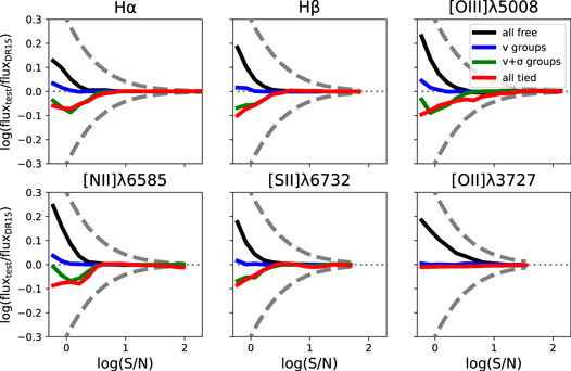
Figure 18. Median of the ratio of emission-line fluxes (in dex) obtained between runs with different tying prescriptions for the emission lines and DR15 as a function of S/N. The gray dashed lines correspond to the scatter expected considering the random errors. The largest systematic discrepancies between the tying strategy implemented in DR15 and the other test runs are found for S/N < 6.
Download figure:
Standard image High-resolution imageFor S/N < 2, the all-free case gives larger fluxes than DR15 for all lines considered. Figure 19 shows a similar plot but for the velocity dispersions, demonstrating that the deviations toward larger fluxes are accompanied by lower sigmas. This may be due to the fact that, when velocities are not tied, the algorithm may be fitting noise spikes at low S/N. These spikes tend to have a width of one pixel, leading to smaller dispersions and higher amplitudes.
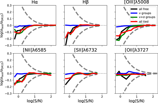
Figure 19. Median ratio of velocity dispersions (in dex) obtained in different test runs (as per legend) and DR15. The gray dashed lines correspond to the scatter expected considering the random errors.
Download figure:
Standard image High-resolution imageThe “v groups” case, where velocities are allowed to vary within emission line groups, is indistinguishable from DR15 in terms of fluxes and sigmas.
Finally, the “v + σ groups” and “all tied” test runs produce marginally lower sigmas and fluxes than DR15.
In Figure 20 we show the velocity difference between DR15 and different test runs for Hα [N ii]λλ 6584 and [O iii]λλ 5007. It is evident that there is no systematic velocity shift if velocities are tied in groups rather than all together. If the velocities are not tied (or tied in groups), the scatter in the resulting velocities with respect to DR15 is comparable to the random error (estimated in DR15) for the metal (both high- and low-ionization) lines, but smaller for the Balmer lines. Overall, the consistency of the velocities determined by following different tying prescriptions validates the DR15 approach and demonstrates that the MaNGA data do not suffer from any detectable systematic in the wavelength calibration (see also Figure 19 of Law et al. 2016), which would necessarily invalidate some of our tying schemes.
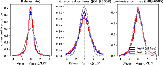
Figure 20. Velocity difference between test runs 0 and 1 and DR15 normalized by the error. A normalized Gaussian is shown in dashed gray for comparison.
Download figure:
Standard image High-resolution imageFinally, in Figure 21 we show the ratio (in dex) between the Hα velocity dispersion and that of other Balmer (in black) and metal (in blue) emission lines as a function of wavelength, after subtracting in quadrature the DR15 estimate of the instrumental velocity dispersion. Only spaxels with S/N > 10 on the specific line are considered. The figure demonstrates that in DR15 the velocity dispersions of different emission lines within the MILES wavelength range are in good agreement with each other, with no significant wavelength-dependent systematic. The largest discrepancies are found in the blue end of the wavelength range, where both [O ii] and Hδ are larger than Hα by 0.07 dex (∼17%) on average.
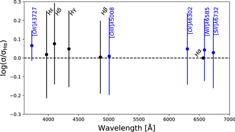
Figure 21. Ratio (in dex) between the intrinsic velocity dispersion of different emission lines with respect to Hα in DR15 as a function of wavelength. The intrinsic (astrophysical) dispersion is measured by subtracting, in quadrature, our estimate of the instrumental velocity dispersion from the measured line velocity dispersion. Balmer lines are represented in black and metal lines in blue. Only spaxels with S/N > 10 in the specific emission line are considered to generate the plot. The error bars represent the 1σ scatter.
Download figure:
Standard image High-resolution image6. Recommendations and Future Work
6.1. Recommendations on the Use of the DR15 DAP Data Products
Here we briefly summarize our recommendations for usage of the DAP DR15 output regarding emission lines.
Users whose science goal would benefit from the best spatial resolution afforded by MaNGA should use the output from the hybrid binning scheme contained in the HYB10-GAU-MILESHC directory. If, on the other hand, one requires the emission-line properties to be computed on the same (Voronoi) binning scheme as the continuum, the output in VOR10-GAU-MILESHC should be used instead.
All of the emission-line maps are included as extensions in the DAP MAPS files. Each extension corresponds to a 3D array, where two dimensions correspond to the on-sky spatial pixels and the third dimension allows the user to choose a specific emission line. These extensions can be opened with a standard fits viewer (e.g., DS9,27 QFitsView28 ) and appear as a datacube. The correspondence between the index in the MAPS file extension and the line name is given in the extension header. A practical example of how to perform this association in an automatic fashion in python is given below.
| # Declare a function that creates a dictionary for the columns in the multi-channel extensions |
| def column_dictionary(hdu, ext): |
| columndict = {} |
| for k, v in hdu[ext].header.items(): |
| if k[0] == ‘C’: |
| try: |
| # the −1 makes the indices zero-based as opposed to 1-based |
| i = int(k[1:])−1 |
| except ValueError: |
| continue |
| columndict[v] = i |
| return columndict |
| # end of the function declaration |
Download table as: ASCIITypeset image
We strongly encourage users to take close consideration of the masks provided in the MAPS file. In the python programming language, masked arrays, as implemented in the numpy package, are particularly suitable for the task of manipulating data with associated mask information. Masked arrays allow one to perform arithmetic and other simple operations (like taking a median) while automatically ignoring the masked pixels. The code example below provides an example of how to obtain the Hα flux map from the DAP MAPS file and encode it into a numpy masked array.
| import numpy as np |
| from astropy.io import fits |
| # open the maps file (hybrid binning scheme) for galaxy |
| 8138--12704 |
| hdu = |
| fits.open(‘manga-8138-12704-MAPS-HYB10-GAU-MILESHC.fits.gz’) |
| emline = column_dictionary(hdu, ’EMLINE_GFLUX’) |
| # get the Ha map as a masked array |
| flux_Ha = np.ma.MaskedArray( |
| hdu[‘EMLINE_GFLUX’].data[emline[‘Ha-6564’],:,:], |
| mask = hdu[’EMLINE_GFLUX_MASK’].data[emline[’Ha-6564’],:,:] |
| >0) |
Download table as: ASCIITypeset image
Users interested in a comprehensive software framework in the python language to access and manipulate the MaNGA data are encouraged to use our purpose-built Marvin package (Cherinka et al. 2019). Visualization tools for the DAP data products are also directly available on the Marvin web interface at https://dr15.sdss.org/marvin/.
Finally, we warn users of the following bugs that were discovered in the DR15 DAP output. These problems have already been resolved at the software level, and the DAP output will be corrected in the next data release.
- 1.The [O ii]λλ 3727,29 velocity-dispersion masks and errors are incorrect in DR15. In particular, the vast majority of spaxels in the velocity-dispersion maps of [O ii] are masked in DR15 because of a bug. The maps of the velocity dispersions themselves are, however, correct. We therefore recommend ignoring the mask extensions for the [O ii]λλ 3727,29 line velocity dispersions and applying the Hα velocity dispersion masks instead. Unfortunately, the same bug caused the inverse variance extensions for the [O ii] lines to be filled with zeros. This has been fixed for future releases, but for DR15, uncertainties for the [O ii] velocity dispersions are not available.
- 2.The Hζ line parameters are unreliable in DR15. This is due to a blend with the nearby He i line at 3889.749 Å (vacuum) that was not included in the line list for DR15, but will be included in future releases. We recommend against use of this line in DR15.
6.2. Future Work
There are many ways to improve on DR15 with respect to the emission-line properties. First, we would like to transition away from MILES-HC toward a stellar library derived from MaStar spectra (Yan et al. 2018). MaStar is a new library of stellar spectra observed with the MaNGA instrument suite at APO and offers several advantages over MILES, in terms of its carefully controlled flux calibration, wider coverage in terms of stellar parameters, wider wavelength range, and LSF similar to the MaNGA galaxy spectra.
The generation of a hierarchically clustered set of MaStar spectra for kinematics extraction and the production of a new generation of SSP templates based on MaStar spectra are currently being pursued by the MaNGA team. We anticipate incorporating a “MaStar-HC” library or a set of MaStar-based SSP templates for the simultaneous fitting of continuum and emission lines in the second fitting stage of the DAP. The use of continuum templates with wider wavelength coverage would also allow us to provide accurate modeling of the continuum for the [S iii]λ8831,9071 9533 lines in the near-infrared, which are sensitive tracers of the ionization parameter of the ISM (Kewley & Dopita 2002).
A detailed characterization of the MaNGA LSF is currently underway and will be described in a forthcoming publication. Nonetheless, the results presented in Section 5.3, and Figure 21 in particular, demonstrate that the current estimate of the MaNGA LSF is sufficiently accurate to move toward a tying scheme where both velocity and velocity dispersion are tied for physically motivated groups of lines. We anticipate that the next MaNGA data release will adopt either the “all tied” or the “v + σ groups” tying approach described in Section 5.3.
Further improvements may include a treatment of multi-Gaussian kinematic components and broad emission lines in AGNs. While automatically detecting very broad emission lines (σ > 1000 km s−1) is a relatively simple task, characterizing the significance of line asymmetries or additional kinematic components for millions of low-S/N, medium-resolution MaNGA spaxels represents a significant task, likely to remain outside the scope of a general-purpose data analysis pipeline like the DAP. Gallagher et al. (2019) describe the first attempt at this type of analysis on the MaNGA data.
Given the timescale of the SDSS-IV project, which is scheduled to terminate data collection in 2020, we do not expect further substantial project-led developments of the MaNGA DAP. Members of the astronomical community interested in adapting the MaNGA DAP to their own specific data format and scientific interests are welcome to make use of the DAP source code, which is publicly released on GitHub.29
7. Summary and Conclusions
In this paper we have tested the algorithmic choices and output produced by the MaNGA DAP with regard to the quality of the stellar-continuum modeling and the determination of emission-line fluxes and kinematics. We have further described and assessed the choices made for SDSS DR15, which corresponds to the first public release of DAP data products. We hope that the analysis presented in this paper will serve as a reference for the community interested in the intricacies of spectral fitting and to those who wish to use the high-level data products from the MaNGA survey released in DR15.
The main conclusions of this work are summarized below:
- 1.We derive a tight relationship between the amplitude-to-noise and the ratio between measured flux and flux error (S/N). We therefore consider the S/N as an appropriate metric for emission lines in MaNGA. For S/N < 30, emission lines are statistically well fit by the DAP, with a χ2/dof ∼ 0.8. An increase in χ2/dof is observed at higher S/N, which we expect is associated with template mismatch (i.e., non-Gaussian line profiles are more well measured at high S/N). By comparing Gaussian and nonparametric (summed) fluxes, we conclude that, despite the increase in χ2/dof at high S/N, our Gaussian line fluxes in that regime are accurate.
- 2.We generate mock datacubes with realistic error prescriptions and demonstrate that the estimated errors for flux and velocity dispersion behave in a statistically correct way down to S/N ∼ 1.5. Errors in the velocity are underestimated for S/N < 10, and we provide an empirical formula (Equation (3)) to correct this underestimation. We note that applying this correction is the responsibility of the user, because the correction is not automatically applied to the DAP output.
- 3.We analyze the error statistics from repeat observations. The conclusions largely support what is observed for the idealized simulations. In addition, repeat observations show an underestimation of the errors in the high-S/N regime. We have demonstrated that this trend can be entirely explained by small astrometric errors in individual exposures, which are consistent with the uncertainties derived by the MaNGA astrometry registration routine. In light of this, we leave it up to the user to consider whether adding this extra error contribution is advisable for their specific science goals.
- 4.We tested how well the hierarchically clustered MILES library (MILES-HC), employed in DR15, can be used to fit very young stellar populations (taken from the BC03 SSP library). MILES-HC can reproduce the correct spectral shape even without the use of polynomials and most of the Balmer absorption lines for ages older than 25 Myr. Helium absorption lines and Balmer lines in a 5-Myr-old population are more difficult to reproduce, even when allowing the introduction of polynomials.
- 5.We have studied how the emission-line fluxes may differ if the continuum is fit with a set of different SSP template libraries (M11-MILES, BC03, and MIUSCAT). We find large discrepancies in the recovered fluxes (>0.1 dex) for S/N < 10. Metal lines are less affected; however, [N ii] seems to be affected in a coherent fashion with nearby Hα. These differences in flux can cause larger discrepancies in derived line ratios, extinction correction, and metallicity-sensitive indicators. We find discrepancies of 0.1 dex for the O3N2 and log(R23) metallicity-sensitive indices even for EW(Hα) > 6 Å, where flux from H ii regions generally dominates over diffuse ionized gas and LIER emission. The choice of template library appears therefore to be the largest source of systematic error studied in this paper.
- 6.By generating mock cubes with a particular template library and using an alternative library to fit them, we demonstrate that the derived emission-line errors remain statistically accurate even in the presence of template mismatch.
- 7.There is no evidence pointing toward inaccuracies in the MaNGA flux calibration in the MILES wavelength range, although there is a hint of a red upturn for λ > 9000, which we have not investigated further because this wavelength range is not fit in DR15. The small deviations (<10%) from the smooth curves expected for a physical extinction model present in the DR15 polynomials are probably due to inaccuracies in the MILES library flux calibration.
- 8.Simultaneously fitting the continuum and emission lines, as done in the DAP, has a minor effect on the Balmer line fluxes (<2% on Hα, although the effect can be larger on the higher-order Balmer lines) and no measurable effect on strong metal lines. The use of additive, rather than multiplicative, polynomials leads to discrepancies in others areas of the spectrum, but still at the few-percent level.
- 9.We have investigated different tying strategies and compared them with the approach followed in DR15, in which all lines were fit with a common velocity and independent velocity dispersions. Large differences (>0.1 dex) are found comparing DR15 and the case where all kinematic components are left free, but only for S/N < 2. Treating all velocities independently or tying velocities of all the lines, or groups of lines, with similar ionization potential does not lead to any systematic changes in the best-fit velocity. Considering the DR15 determination of the instrumental dispersion at the position of different emission lines, velocity dispersions of different lines agree with Hα on average to better than 0.07 dex across the full MILES wavelength range. These facts demonstrate the accuracy of the MaNGA wavelength calibration and LSF determination.
The data products generated by the MaNGA DAP are made publicly available at http://www.sdss.org/dr15/manga/, while the DAP source code can be accessed via GitHub at https://github.com/sdss/mangadap.
We thank the anonymous referee for the enlightening and supportive report. M.A.B. acknowledges NSF Award AST-1517006. C.A.T. acknowledges NSF Award AST-1554877. S.F.S. acknowledges the following projects for their support: CONACYT FC-2016-01-1916, CONACYT BC-285080, and PAPIIT IN100519. M.C. acknowledges support from a Royal Society University Research Fellowship. R.Y. acknowledges support by NSF award AST-1715898. This work makes use of data from SDSS-IV. Funding for SDSS has been provided by the Alfred P. Sloan Foundation and Participating Institutions. Additional funding toward SDSS-IV has been provided by the U.S. Department of Energy Office of Science. SDSS-IV acknowledges support and resources from the Center for High-Performance Computing at the University of Utah. The SDSS website is www.sdss.org. This research made use of Marvin, a core Python package and web framework for MaNGA data, developed by Brian Cherinka, José Sánchez-Gallego, and Brett Andrews (Cherinka et al. 2019). SDSS-IV is managed by the Astrophysical Research Consortium for the Participating Institutions of the SDSS Collaboration including the Brazilian Participation Group, the Carnegie Institution for Science, Carnegie Mellon University, the Chilean Participation Group, the French Participation Group, Harvard-Smithsonian Center for Astrophysics, Instituto de Astrofísica de Canarias, The Johns Hopkins University, Kavli Institute for the Physics and Mathematics of the Universe (IPMU)/University of Tokyo, Lawrence Berkeley National Laboratory, Leibniz Institut für Astrophysik Potsdam (AIP), Max-Planck-Institut für Astronomie (MPIA Heidelberg), Max-Planck-Institut für Astrophysik (MPA Garching), Max-Planck-Institut für Extraterrestrische Physik (MPE), National Astronomical Observatory of China, New Mexico State University, New York University, University of Notre Dame, Observatário Nacional/MCTI, The Ohio State University, Pennsylvania State University, Shanghai Astronomical Observatory, United Kingdom Participation Group, Universidad Nacional Autónoma de México, University of Arizona, University of Colorado Boulder, University of Oxford, University of Portsmouth, University of Utah, University of Virginia, University of Washington, University of Wisconsin, Vanderbilt University, and Yale University.
The MaNGA data used in this work are publicly available at http://www.sdss.org/dr15/manga/manga-data/.
Appendix: Comparison with Pipe3D
We have shown that the extraction of emission-line fluxes by the DAP is statistically robust between repeat observations, and that the estimated errors on the flux are well determined down to S/ N = 1.5. However, as we have shown in Sections 3 and 4, systematics may exist in the recovered fluxes of lines based on the choices of continuum model used and other aspects of the fitting methodology. To explore the potential differences that may exist between different fitting routines, we compare some of the derived emission-line properties between the DAP and Pipe3D.
The philosophy behind the fitting of the emission lines differs markedly between the DAP and Pipe3D: while the DAP fits the emission lines with (positive) Gaussian templates simultaneously with the stellar continuum, Pipe3D only fits Gaussians to the strong emission lines. The strong lines are collected into four groups based on their wavelengths, and the velocities of these lines within these groups are kinematically tied. These groups are (1) the [O ii] λλ 3727,3729 doublet; (2) Hβ and [O iii]λλ 4959, 5007; (3) [N ii]λλ 6548,84 and Hα; and (4) [S ii] λλ 6717,31. For the weaker emission lines, Pipe3D performs a moment-based analysis to numerically integrate the weak emission lines and uses a Monte Carlo method to estimate the errors (Sánchez et al. 2016b, Sections 3.5–3.6). This fitting algorithm can return a negative value for low-S/N spectra.
While the DAP fits the stellar component of the spectrum using the MILES-HC library, Pipe3D models the stellar light with a set of 156 SSP models that the authors refer to as the GSD156 library (Cid Fernandes et al. 2013). This set of templates includes the Granada models of González Delgado et al. (2005) for stellar populations younger than 63 Myr and the Vazdekis et al. (2010) models for older stellar populations. The GSD156 library covers a grid in age and metallicity, with ages ranging from 1 Myr to 14.1 Gyr and covering four values of metallicity (Z/Z⊙ = 0.2, 0.4, 1.0, and 1.5).
A.1. Comparison of Line Fluxes
We first compare the fluxes between Pipe3D and the DAP for a set of strong lines ([O ii]λλ 3727,3729, Hβ, [O iii]λ 5007, Hα, [N ii]λ 6584, and [S ii]λ 6731). We perform this comparison using a large sample of 3 × 10⁶ spaxels from 4565 datacubes. We compare the ratio of the fluxes from each suite pipeline as a function of the DAP S/N in Figure 22. At high S/N, the line fluxes agree to within 0.02 dex, or ∼5%. For S/N < 10, the DAP consistently estimates emission lines to be brighter than Pipe3D. For Hα the median of this effect is of order 0.05 dex (12%) for 3 < S/N < 10 and as much as 0.12 dex (28%) for [N ii]λ 6584 in the same S/N range. Hβ behaves differently from the other lines tested, as the DAP reports lower average fluxes compared to Pipe3D at low S/N. For the Balmer lines, this may be related to the differences in the stellar-absorption-line fits between the two pipelines; however, this explanation seems less likely for the forbidden lines. We note that for weak lines, the DAP stipulation that emission-line fluxes must be positive will introduce a positive bias, which may partially explain the upward skew seen in the distributions for low-S/N lines in Figure 22.
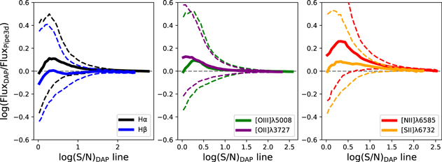
Figure 22. Ratio of emission-line flux as measured by the DAP to the flux measured by Pipe3D as a function of the emission-line S/N (from the DAP). The solid lines represent the median of the distribution, while the dashed lines represent the 16th and 84th percentiles of the distributions.
Download figure:
Standard image High-resolution image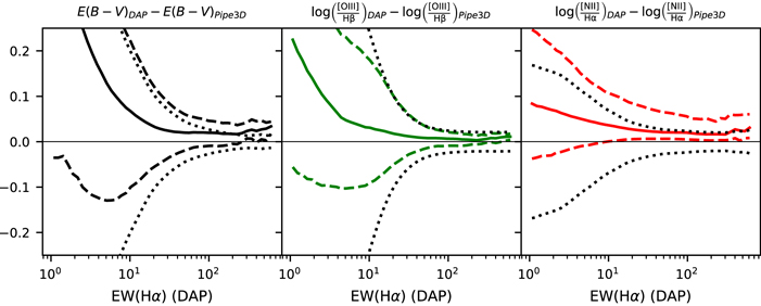
Figure 23. Difference in emission-line ratios as measured by the DAP to those measured by Pipe3D as a function of EW(Hα). The solid lines are the median difference, and the dashed lines are the 16th and 84th percentiles of the distribution. While skewed upward at low EW, the distributions of  and [O iii]/Hβ are consistent within the measurement uncertainties. This is not true for [N ii]/Hα, for which the DAP has measured a higher value, even at high Hα EW.
Download figure:
Standard image High-resolution imageA.2. Effect on Line Ratios and Metallicity
The small systematic offsets observed in the line fluxes can be enhanced when one computes some commonly used line ratios. Given the importance of establishing the consistency of these higher-level measurements, we compare the values of  , [N ii]/Hα, and [O iii]/Hβ obtained by DAP and Pipe3D as a function of EW(Hα) (see Figure 23).
For EW(Hα) > 20 Å, the line ratios considered are in reasonable agreement between the two pipelines, although both for  and [N ii]/Hα a roughly constant systematic offset (∼0.02 dex) is observed even at high EW. The agreement considerably worsens at low EW. Two main differences exist between the methodologies of Pipe3D and the DAP that might influence the fluxes of the emission lines. These two pipelines use different template libraries to fit the stellar continua. This difference can result in differences in line fluxes, particularly at low EW. Since the [N ii]λ 6584 line is adjacent to
  , the features in the wings of the absorption line can impact the measured flux of the [N ii]λ 6584 line, particularly in spectra with high stellar velocity dispersion.
The reasons for this behavior are explored in the left-hand panel of Figure 24, where we show four example spectra and the stellar-continuum fits performed by the DAP and Pipe3D. These spectra were chosen to cover a range of [N ii] EW and σ⋆ values. In these examples, we can see that differences in the adopted continuum model can have an effect on the flux in the emission lines, even in the spectral region around the forbidden lines. For the highest stellar velocity dispersions, the Hα absorption can spread underneath the [N ii] lines, leading to an overestimate of the [N ii] flux.
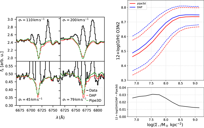
Figure 24. On the left we show example fits performed by the DAP and Pipe3D around the [N ii]/Hα region. Systematic differences in the absorption-line profile can extend underneath the [N ii] emission line. This may explain the systematic differences in the [N ii] fluxes between pipelines. On the right is the resolved mass–metallicity relation, computed using the O3N2 diagnostic and the Pettini & Pagel (2004) metallicity calibration, using the DAP and Pipe3D line fluxes for single spaxels in the MaNGA survey. The stellar mass surface density ( ) is always taken from the Pipe3D VAC. Only spaxels with S/N > 3 on the relevant line fluxes and classified as star-forming in the BPT diagram are plotted. The solid lines represent the median relations, and the dashed lines are the 16th and 84th percentiles. The resolved mass–metallicity relations obtained from the two different pipelines are in good agreement with regards to the shape of the relation, despite showing a systematic offset in metallicity of the order of 0.01–0.03 dex, as shown in the bottom panel.
Download figure:
Standard image High-resolution imageThe potential effect on a specific scientific result of the discrepancy between the DAP and Pipe3D fluxes is illustrated in Figure 24, right panel, where we show the resolved mass–metallicity relation obtained from the two pipelines using the O3N2 metallicity calibrator and the Pettini & Pagel (2004) calibration. We consider only spaxels classified as star-forming using the Kewley et al. (2001) line in the [S ii] BPT diagram. All spaxels with S/N < 3 for the emission lines required for the O3N2 diagnostic are excluded. The stellar mass surface density values for each spaxel are taken from the Pipe3D VAC. These values are corrected for the effect of dust extinction, but not for the potential effect of galaxy inclination. The shape of the resulting resolved mass–metallicity relation agrees well with previous studies based on a smaller sample of MaNGA galaxies (Barrera-Ballesteros et al. 2016). We note, moreover, that the determinations obtained from both pipelines are in very good agreement with regards to the shape of the relation, despite a systematic shift in the median metallicity. This shift is of the order of 0.03 dex at low metallicity, decreasing to 0.01 dex at high metallicity. Since the systematics associated with metallicity calibrations are larger than this offset, we consider that the choice of pipeline does not significantly affect this science case.
The comparison performed in this appendix highlights the difficulties in measuring the strengths of emission lines in galaxy spectra. Systematic differences in the derived fluxes for strong, high-EW lines are within a few percent for the majority of the lines examined here. We have checked that the effect on the resolved mass–metallicity relation is small (0.03 dex at most) but clearly systematic. However, caution should be taken not to overinterpret fluxes and flux ratios of emission lines, particularly in the regime of low line EW and for weak lines that are likely to be severely affected by the quality of the continuum subtraction.
Footnotes
- 15
Available at https://pypi.org/project/ppxf/.
- 16
Available at https://pypi.org/project/vorbin/.
- 17
Tying the [O ii]λλ 3727,29 doublet is particularly important because it is unresolved at the MaNGA spectral resolution, and large degeneracies in the fit would result otherwise.
- 18
For the data model of the MAPS file, see https://data.sdss.org/datamodel/files/MANGA_SPECTRO_ANALYSIS/DRPVER/DAPVER/DAPTYPE/PLATE/IFU/manga-MAPS-DAPTYPE.html and Section 11.1 and Table 4 of Westfall et al. (2019).
- 19
For the model LOGCUBE data model, see https://data.sdss.org/datamodel/files/MANGA_SPECTRO_ANALYSIS/DRPVER/DAPVER/DAPTYPE/PLATE/IFU/manga-LOGCUBE-DAPTYPE.html and Section 11.2 and Table 5 of Westfall et al. (2019).
- 20
The same side bands are used to determine the continuum term in the computation of EW and are listed in Table 3 of Westfall et al. (2019).
- 21
Forty-three galaxies have been observed twice, 12 have been observed three times, and one has been observed four times, for a total of 70 pairs of galaxies with repeat observations.
- 22
- 23
- 24
- 25
- 26
We recall here that at this stage the data have already been corrected for Galactic foreground extinction.
- 27
- 28
- 29